Lesson 07: Edge Detection

Edge detection is one of the most fundamental operations in computer vision. Edges mark boundaries between regions of different intensity — and those boundaries often correspond to object outlines, surface discontinuities, or illumination changes. In this lesson, we will cover three key techniques: Sobel, Laplacian, and Canny edge detection.

1. What Is an Edge?

An edge in an image is a location where the pixel intensity changes rapidly. Mathematically, this corresponds to a high value of the image gradient — the first derivative of the image intensity function.

\text{Gradient} = \nabla I = \left(\frac{\partial I}{\partial x}, \frac{\partial I}{\partial y}\right)

Edge detectors approximate this gradient using convolution kernels.

2. Sobel Edge Detector

The Sobel operator approximates the gradient of the image intensity using two 3×3 kernels — one for horizontal changes (Gx) and one for vertical changes (Gy):

G_x = \begin{bmatrix} -1 & 0 & 1 \\ -2 & 0 & 2 \\ -1 & 0 & 1 \end{bmatrix}, \quad G_y = \begin{bmatrix} -1 & -2 & -1 \\ 0 & 0 & 0 \\ 1 & 2 & 1 \end{bmatrix}

The magnitude of the gradient is:

G = \sqrt{G_x^2 + G_y^2}

import cv2
import numpy as np

img = cv2.imread("image.jpg")
gray = cv2.cvtColor(img, cv2.COLOR_BGR2GRAY)

# Compute Sobel gradients
sobel_x = cv2.Sobel(gray, cv2.CV_64F, 1, 0, ksize=3)
sobel_y = cv2.Sobel(gray, cv2.CV_64F, 0, 1, ksize=3)

# Combine and convert back to 8-bit
sobel_combined = cv2.magnitude(sobel_x, sobel_y)
sobel_combined = np.uint8(np.clip(sobel_combined, 0, 255))

cv2.imshow("Sobel X", np.uint8(np.abs(sobel_x)))
cv2.imshow("Sobel Y", np.uint8(np.abs(sobel_y)))
cv2.imshow("Sobel Combined", sobel_combined)
cv2.waitKey(0)
cv2.destroyAllWindows()

Parameters for cv2.Sobel():

src – input image (must be grayscale for most uses)
ddepth – output depth (cv2.CV_64F avoids clipping negative values)
dx, dy – order of derivative in x and y directions
ksize – size of the Sobel kernel (1, 3, 5, or 7)

Tip: Use cv2.CV_64F as the depth to capture both positive and negative gradients. Converting directly to uint8 will lose negative edges.

3. Laplacian Edge Detector

The Laplacian operator computes the second derivative of the image, highlighting regions of rapid intensity change in all directions at once:

\nabla^2 I = \frac{\partial^2 I}{\partial x^2} + \frac{\partial^2 I}{\partial y^2}

import cv2
import numpy as np

img = cv2.imread("image.jpg")
gray = cv2.cvtColor(img, cv2.COLOR_BGR2GRAY)

# Apply Gaussian blur first to reduce noise sensitivity
blurred = cv2.GaussianBlur(gray, (5, 5), 0)

laplacian = cv2.Laplacian(blurred, cv2.CV_64F)
laplacian_abs = np.uint8(np.absolute(laplacian))

cv2.imshow("Original", gray)
cv2.imshow("Laplacian", laplacian_abs)
cv2.waitKey(0)
cv2.destroyAllWindows()

The Laplacian is very sensitive to noise, so it is almost always applied after Gaussian blurring.

4. Canny Edge Detector

The Canny edge detector is the most widely used edge detection algorithm in practice. It produces thin, well-localized edges and is robust to noise. It works in four steps:

Noise reduction – Gaussian blur to smooth the image
Gradient computation – Sobel operators to find gradient magnitude and direction
Non-maximum suppression – Thin the edges to 1-pixel width
Hysteresis thresholding – Keep strong edges, trace weak edges connected to strong ones

import cv2

img = cv2.imread("image.jpg")
gray = cv2.cvtColor(img, cv2.COLOR_BGR2GRAY)

# Canny edge detection
edges = cv2.Canny(gray, threshold1=50, threshold2=150)

cv2.imshow("Original", gray)
cv2.imshow("Canny Edges", edges)
cv2.waitKey(0)
cv2.destroyAllWindows()

Parameters for cv2.Canny():

threshold1 – lower threshold for hysteresis; edges below this are discarded
threshold2 – upper threshold; edges above this are definitely kept
Edges between the two thresholds are kept only if connected to a strong edge

Choosing thresholds: A common heuristic is to use a ratio of 1:2 or 1:3 between the low and high thresholds. You can also use Otsu's threshold as a starting point:

import cv2
import numpy as np

img = cv2.imread("image.jpg")
gray = cv2.cvtColor(img, cv2.COLOR_BGR2GRAY)

# Use Otsu's threshold to auto-select Canny thresholds
otsu_thresh, _ = cv2.threshold(gray, 0, 255, cv2.THRESH_BINARY + cv2.THRESH_OTSU)
edges = cv2.Canny(gray, otsu_thresh * 0.5, otsu_thresh)

cv2.imshow("Auto-threshold Canny", edges)
cv2.waitKey(0)
cv2.destroyAllWindows()

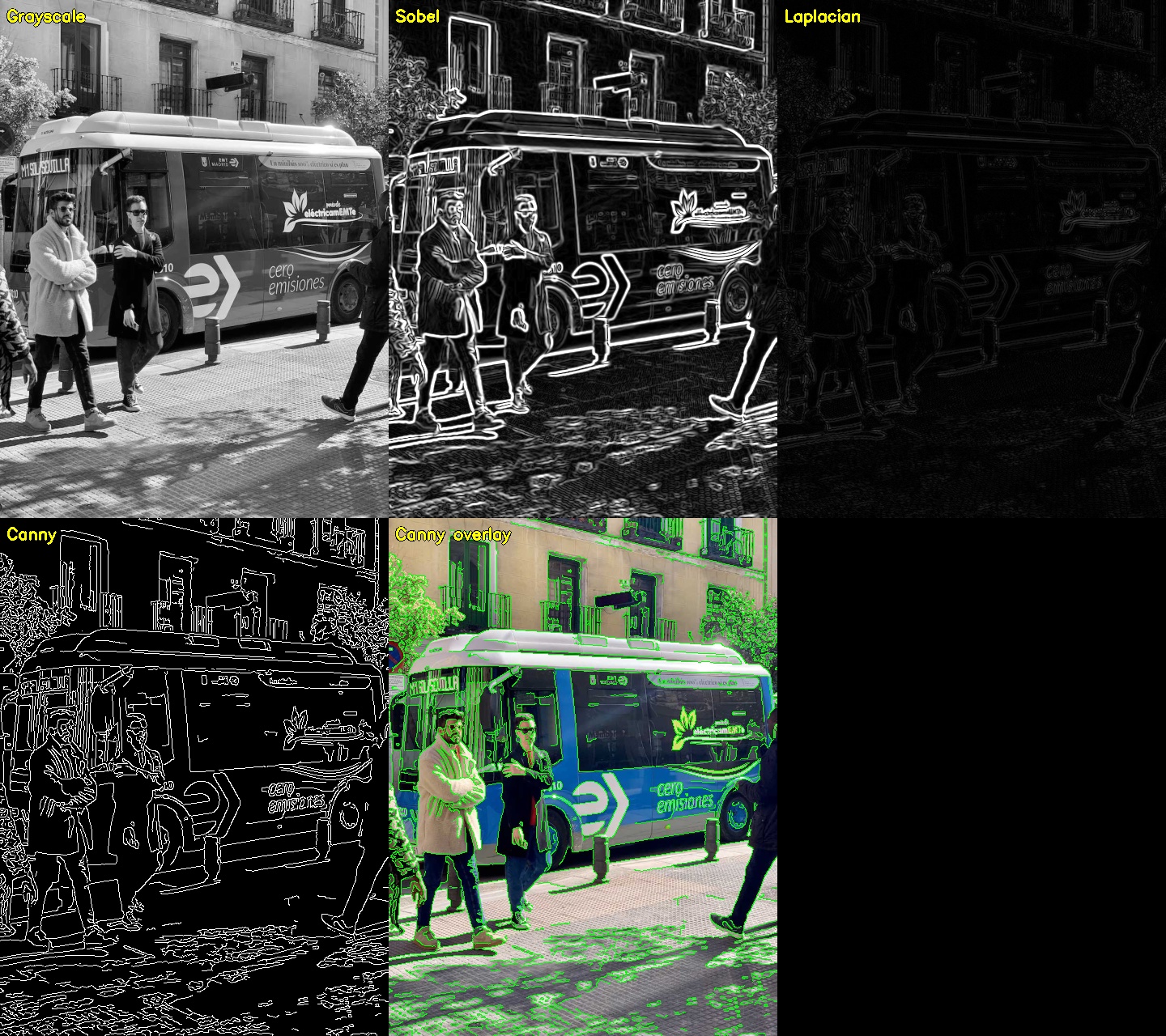
5. Comparing the Three Methods

import cv2
import numpy as np

img = cv2.imread("image.jpg")
gray = cv2.cvtColor(img, cv2.COLOR_BGR2GRAY)
blurred = cv2.GaussianBlur(gray, (5, 5), 0)

# Sobel
sobel_x = cv2.Sobel(blurred, cv2.CV_64F, 1, 0, ksize=3)
sobel_y = cv2.Sobel(blurred, cv2.CV_64F, 0, 1, ksize=3)
sobel = np.uint8(np.clip(cv2.magnitude(sobel_x, sobel_y), 0, 255))

# Laplacian
laplacian = np.uint8(np.absolute(cv2.Laplacian(blurred, cv2.CV_64F)))

# Canny
canny = cv2.Canny(blurred, 50, 150)

# Stack horizontally for comparison
comparison = np.hstack([sobel, laplacian, canny])
cv2.imshow("Sobel | Laplacian | Canny", comparison)
cv2.waitKey(0)
cv2.destroyAllWindows()

Method	Strengths	Weaknesses
Sobel	Simple, fast, directional	Thick edges, sensitive to noise
Laplacian	Detects edges in all directions	Very noise-sensitive
Canny	Thin edges, robust, widely used	Two thresholds to tune

6. Practical Example: Outline Detection

import cv2

img = cv2.imread("image.jpg")
gray = cv2.cvtColor(img, cv2.COLOR_BGR2GRAY)

# Detect edges
edges = cv2.Canny(gray, 50, 150)

# Overlay edges in green on the original image
output = img.copy()
output[edges != 0] = [0, 255, 0]

cv2.imshow("Edge Overlay", output)
cv2.waitKey(0)
cv2.destroyAllWindows()

Test Images

You can run edge detection on a publicly available image without needing local files. The bicycle photo below is a good test case because it contains many well-defined geometric edges — wheel rims, frame tubes, spokes, and handlebars.

import cv2
import numpy as np
import urllib.request

# Download the bicycle image from Wikimedia Commons
url = "https://upload.wikimedia.org/wikipedia/commons/thumb/3/3f/Bikesgray.jpg/1280px-Bikesgray.jpg"
urllib.request.urlretrieve(url, "bikes.jpg")

img = cv2.imread("bikes.jpg")
gray = cv2.cvtColor(img, cv2.COLOR_BGR2GRAY)
blurred = cv2.GaussianBlur(gray, (5, 5), 0)

# Run all three detectors for comparison
sobel_x = cv2.Sobel(blurred, cv2.CV_64F, 1, 0, ksize=3)
sobel_y = cv2.Sobel(blurred, cv2.CV_64F, 0, 1, ksize=3)
sobel = np.uint8(np.clip(cv2.magnitude(sobel_x, sobel_y), 0, 255))

laplacian = np.uint8(np.absolute(cv2.Laplacian(blurred, cv2.CV_64F)))

canny = cv2.Canny(blurred, threshold1=50, threshold2=150)

# Stack for side-by-side comparison
comparison = np.hstack([sobel, laplacian, canny])
cv2.imshow("Sobel | Laplacian | Canny  (bikes)", comparison)
cv2.waitKey(0)
cv2.destroyAllWindows()

What to expect in the output:

Canny produces the cleanest result on this image: thin, continuous lines tracing the circular wheel rims, the straight diagonal and horizontal frame tubes, and dozens of thin parallel spokes radiating from each hub. The handlebar curves appear as clean arcs.
Sobel shows thicker edges and captures the same structural elements, but with more gradient noise across the tire surfaces and background.
Laplacian is the noisiest of the three — it reacts to fine texture in the tires and gravel background, making it harder to isolate the structural edges.

The bicycle image is particularly useful for edge detection study because it contains a mix of: circles (rims), straight lines (frame, forks), thin parallel curves (spokes), and gradual curves (handlebars) — covering most real-world edge types in one image.

Edge detection comparison: Grayscale → Sobel → Laplacian → Canny → Canny overlay on original

Conclusion

Edge detection is a critical preprocessing step in many computer vision pipelines — from object detection to image segmentation. The Canny detector is the go-to choice in most situations due to its accuracy and noise robustness. In the next lesson, we will look at thresholding and morphological operations, which are often used alongside edge detection to isolate and refine regions of interest.