Lesson 09: Contours & Shape Analysis

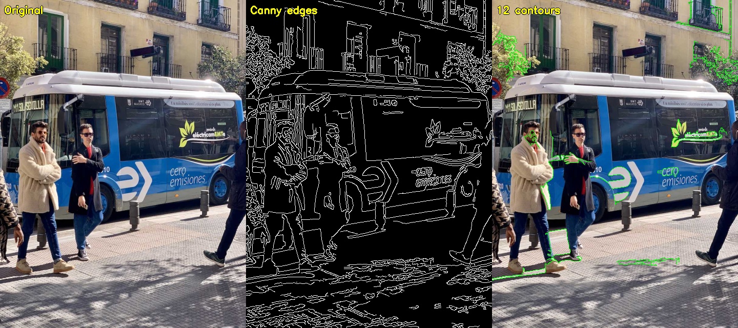
Contours are curves that join continuous points along a boundary with the same intensity. In practice, they are the outlines of objects in binary images — and analyzing them lets you count objects, measure their size, classify their shape, and much more.

1. Finding Contours

cv2.findContours() extracts contours from a binary image. Always apply thresholding or edge detection first.

import cv2
import numpy as np

img = cv2.imread("shapes.jpg")
gray = cv2.cvtColor(img, cv2.COLOR_BGR2GRAY)
_, binary = cv2.threshold(gray, 127, 255, cv2.THRESH_BINARY)

# Find contours
contours, hierarchy = cv2.findContours(
    binary,
    cv2.RETR_EXTERNAL,     # retrieval mode
    cv2.CHAIN_APPROX_SIMPLE  # approximation method
)

print(f"Found {len(contours)} contours")

Retrieval modes:

Mode	Description
`RETR_EXTERNAL`	Only outermost contours
`RETR_LIST`	All contours, no hierarchy
`RETR_CCOMP`	Two-level hierarchy (outer + holes)
`RETR_TREE`	Full hierarchy

Approximation methods:

Method	Description
`CHAIN_APPROX_NONE`	All contour points
`CHAIN_APPROX_SIMPLE`	Compress horizontal/vertical/diagonal segments
`CHAIN_APPROX_TC89_L1`	Teh-Chin chain approximation

OpenCV 4.x note: cv2.findContours() returns only 2 values (contours, hierarchy) — in OpenCV 3.x it returned 3. Make sure not to unpack 3 values if you're using OpenCV 4.

2. Drawing Contours

import cv2
import numpy as np

img = cv2.imread("shapes.jpg")
gray = cv2.cvtColor(img, cv2.COLOR_BGR2GRAY)
_, binary = cv2.threshold(gray, 127, 255, cv2.THRESH_BINARY)
contours, _ = cv2.findContours(binary, cv2.RETR_EXTERNAL, cv2.CHAIN_APPROX_SIMPLE)

output = img.copy()

# Draw all contours in green
cv2.drawContours(output, contours, -1, (0, 255, 0), 2)

# Draw only the first contour in red
if contours:
    cv2.drawContours(output, contours, 0, (0, 0, 255), 3)

cv2.imshow("Contours", output)
cv2.waitKey(0)
cv2.destroyAllWindows()

3. Contour Properties

Area and Perimeter

import cv2
import numpy as np

img = cv2.imread("shapes.jpg")
gray = cv2.cvtColor(img, cv2.COLOR_BGR2GRAY)
_, binary = cv2.threshold(gray, 127, 255, cv2.THRESH_BINARY)
contours, _ = cv2.findContours(binary, cv2.RETR_EXTERNAL, cv2.CHAIN_APPROX_SIMPLE)

for i, cnt in enumerate(contours):
    area = cv2.contourArea(cnt)
    perimeter = cv2.arcLength(cnt, closed=True)
    print(f"Contour {i}: area={area:.1f}, perimeter={perimeter:.1f}")

Bounding Boxes

import cv2

img = cv2.imread("shapes.jpg")
gray = cv2.cvtColor(img, cv2.COLOR_BGR2GRAY)
_, binary = cv2.threshold(gray, 127, 255, cv2.THRESH_BINARY)
contours, _ = cv2.findContours(binary, cv2.RETR_EXTERNAL, cv2.CHAIN_APPROX_SIMPLE)

output = img.copy()
for cnt in contours:
    # Axis-aligned bounding rectangle
    x, y, w, h = cv2.boundingRect(cnt)
    cv2.rectangle(output, (x, y), (x + w, y + h), (0, 255, 0), 2)

    # Minimum area rotated bounding rectangle
    rect = cv2.minAreaRect(cnt)
    box = cv2.boxPoints(rect)
    box = box.astype(int)
    cv2.drawContours(output, [box], 0, (0, 0, 255), 2)

    # Minimum enclosing circle
    (cx, cy), radius = cv2.minEnclosingCircle(cnt)
    cv2.circle(output, (int(cx), int(cy)), int(radius), (255, 0, 0), 2)

cv2.imshow("Bounding Shapes", output)
cv2.waitKey(0)
cv2.destroyAllWindows()

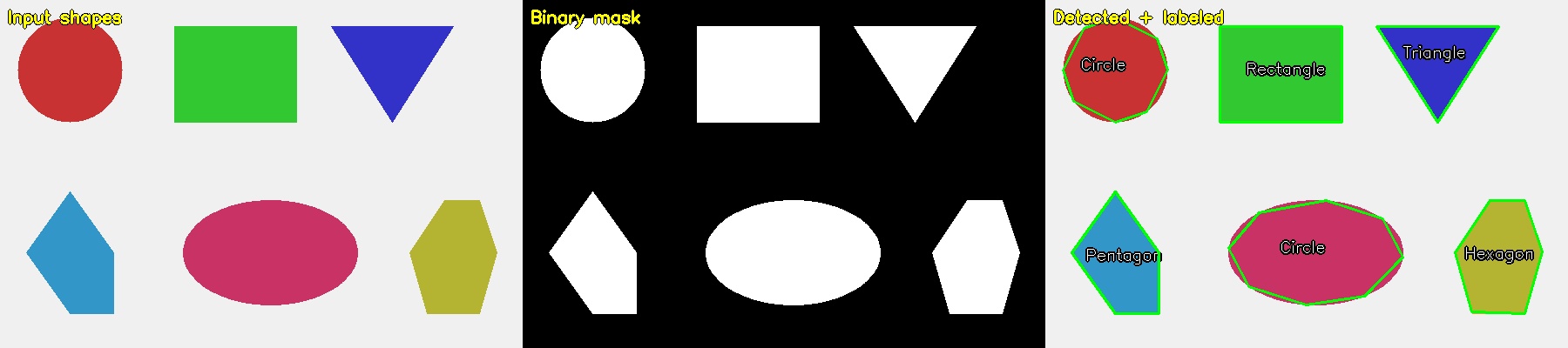
4. Shape Classification with Contour Approximation

Contour approximation reduces the number of points in a contour while preserving its shape. You can use this to classify simple geometric shapes.

import cv2
import numpy as np

img = cv2.imread("shapes.jpg")
gray = cv2.cvtColor(img, cv2.COLOR_BGR2GRAY)
blurred = cv2.GaussianBlur(gray, (5, 5), 0)
_, binary = cv2.threshold(blurred, 60, 255, cv2.THRESH_BINARY)
contours, _ = cv2.findContours(binary, cv2.RETR_EXTERNAL, cv2.CHAIN_APPROX_SIMPLE)

output = img.copy()
for cnt in contours:
    # Skip very small contours (noise)
    if cv2.contourArea(cnt) < 500:
        continue

    # Approximate the contour to a polygon
    epsilon = 0.02 * cv2.arcLength(cnt, True)
    approx = cv2.approxPolyDP(cnt, epsilon, True)
    num_vertices = len(approx)

    # Classify by number of vertices
    if num_vertices == 3:
        shape = "Triangle"
    elif num_vertices == 4:
        x, y, w, h = cv2.boundingRect(approx)
        aspect_ratio = w / float(h)
        shape = "Square" if 0.9 <= aspect_ratio <= 1.1 else "Rectangle"
    elif num_vertices == 5:
        shape = "Pentagon"
    elif num_vertices == 6:
        shape = "Hexagon"
    else:
        shape = "Circle"

    # Draw and label
    M = cv2.moments(cnt)
    if M["m00"] != 0:
        cx = int(M["m10"] / M["m00"])
        cy = int(M["m01"] / M["m00"])
        cv2.putText(output, shape, (cx - 40, cy), cv2.FONT_HERSHEY_SIMPLEX,
                    0.6, (255, 255, 255), 2)
    cv2.drawContours(output, [approx], -1, (0, 255, 0), 2)

cv2.imshow("Shape Classification", output)
cv2.waitKey(0)
cv2.destroyAllWindows()

5. Moments and Centroid

Image moments describe the shape of a contour. The centroid (center of mass) is the most commonly used:

c\_x = \frac{M\_{10}}{M\_{00}}, \quad c\_y = \frac{M\_{01}}{M\_{00}}

import cv2

img = cv2.imread("shapes.jpg")
gray = cv2.cvtColor(img, cv2.COLOR_BGR2GRAY)
_, binary = cv2.threshold(gray, 127, 255, cv2.THRESH_BINARY)
contours, _ = cv2.findContours(binary, cv2.RETR_EXTERNAL, cv2.CHAIN_APPROX_SIMPLE)

output = img.copy()
for cnt in contours:
    M = cv2.moments(cnt)
    if M["m00"] == 0:
        continue
    cx = int(M["m10"] / M["m00"])
    cy = int(M["m01"] / M["m00"])
    cv2.circle(output, (cx, cy), 5, (0, 0, 255), -1)

cv2.imshow("Centroids", output)
cv2.waitKey(0)
cv2.destroyAllWindows()

6. Convex Hull

The convex hull is the smallest convex polygon that contains a contour. It's useful for detecting convexity defects — like the spaces between fingers in a hand gesture.

import cv2

img = cv2.imread("hand.jpg")
gray = cv2.cvtColor(img, cv2.COLOR_BGR2GRAY)
_, binary = cv2.threshold(gray, 80, 255, cv2.THRESH_BINARY)
contours, _ = cv2.findContours(binary, cv2.RETR_EXTERNAL, cv2.CHAIN_APPROX_SIMPLE)

output = img.copy()
for cnt in contours:
    if cv2.contourArea(cnt) < 1000:
        continue
    hull = cv2.convexHull(cnt)
    cv2.drawContours(output, [hull], -1, (0, 255, 0), 2)

    # Find convexity defects
    hull_indices = cv2.convexHull(cnt, returnPoints=False)
    if len(hull_indices) > 3:
        defects = cv2.convexityDefects(cnt, hull_indices)
        if defects is not None:
            for i in range(defects.shape[0]):
                s, e, f, d = defects[i, 0]
                far = tuple(cnt[f][0])
                # d is depth * 256 — filter small defects
                if d > 10000:
                    cv2.circle(output, far, 5, (0, 0, 255), -1)

cv2.imshow("Convex Hull + Defects", output)
cv2.waitKey(0)
cv2.destroyAllWindows()

7. Filtering Contours by Properties

In real applications you rarely want all contours — use area, aspect ratio, or circularity to filter:

import cv2
import numpy as np

img = cv2.imread("image.jpg")
gray = cv2.cvtColor(img, cv2.COLOR_BGR2GRAY)
_, binary = cv2.threshold(gray, 0, 255, cv2.THRESH_BINARY + cv2.THRESH_OTSU)
contours, _ = cv2.findContours(binary, cv2.RETR_EXTERNAL, cv2.CHAIN_APPROX_SIMPLE)

output = img.copy()
for cnt in contours:
    area = cv2.contourArea(cnt)
    perimeter = cv2.arcLength(cnt, True)

    # Skip tiny contours
    if area < 200:
        continue

    # Circularity: 1.0 = perfect circle
    circularity = (4 * np.pi * area) / (perimeter ** 2) if perimeter > 0 else 0

    # Aspect ratio of bounding rect
    x, y, w, h = cv2.boundingRect(cnt)
    aspect_ratio = w / float(h)

    # Keep only roughly circular objects
    if circularity > 0.7:
        cv2.drawContours(output, [cnt], -1, (0, 255, 0), 2)

cv2.imshow("Filtered Contours", output)
cv2.waitKey(0)
cv2.destroyAllWindows()

8. Practical Example: Colored Shapes PNG

The Wikimedia transparency demonstration image contains solid colored geometric shapes on a transparent (checkerboard) background — a clean test case for contour finding and shape classification.

import cv2
import numpy as np
import urllib.request

# Download the colored shapes PNG
url = "https://upload.wikimedia.org/wikipedia/commons/thumb/4/47/PNG_transparency_demonstration_1.png/280px-PNG_transparency_demonstration_1.png"
urllib.request.urlretrieve(url, "shapes.png")

# Load with alpha channel preserved (IMREAD_UNCHANGED gives BGRA)
img_bgra = cv2.imread("shapes.png", cv2.IMREAD_UNCHANGED)

if img_bgra.shape[2] == 4:
    # Use the alpha channel as a binary mask
    alpha = img_bgra[:, :, 3]
    _, binary = cv2.threshold(alpha, 128, 255, cv2.THRESH_BINARY)
    img_bgr = cv2.cvtColor(img_bgra, cv2.COLOR_BGRA2BGR)
else:
    img_bgr = img_bgra
    gray = cv2.cvtColor(img_bgr, cv2.COLOR_BGR2GRAY)
    _, binary = cv2.threshold(gray, 10, 255, cv2.THRESH_BINARY)

# Find contours on the binary mask
contours, _ = cv2.findContours(binary, cv2.RETR_EXTERNAL, cv2.CHAIN_APPROX_SIMPLE)

print(f"Found {len(contours)} shapes")
# Expected: ~4 distinct shape regions (circle, rounded rectangle, triangle, star-like shape)

output = img_bgr.copy()
for cnt in contours:
    area = cv2.contourArea(cnt)
    if area < 300:
        continue  # skip tiny noise contours

    # Approximate polygon and classify
    epsilon = 0.02 * cv2.arcLength(cnt, True)
    approx = cv2.approxPolyDP(cnt, epsilon, True)
    num_vertices = len(approx)

    if num_vertices == 3:
        shape = "Triangle"
    elif num_vertices == 4:
        x, y, w, h = cv2.boundingRect(approx)
        ar = w / float(h)
        shape = "Square" if 0.9 <= ar <= 1.1 else "Rectangle"
    elif num_vertices == 5:
        shape = "Pentagon"
    elif num_vertices == 6:
        shape = "Hexagon"
    else:
        # Use circularity to distinguish circles from complex shapes
        perimeter = cv2.arcLength(cnt, True)
        circularity = (4 * np.pi * area) / (perimeter ** 2) if perimeter > 0 else 0
        shape = "Circle" if circularity > 0.75 else f"Polygon ({num_vertices}pts)"

    # Draw contour and label
    cv2.drawContours(output, [cnt], -1, (0, 255, 0), 2)
    M = cv2.moments(cnt)
    if M["m00"] != 0:
        cx = int(M["m10"] / M["m00"])
        cy = int(M["m01"] / M["m00"])
        cv2.putText(output, shape, (cx - 40, cy),
                    cv2.FONT_HERSHEY_SIMPLEX, 0.55, (0, 0, 255), 2)
    print(f"  {shape}: area={area:.0f}, vertices={num_vertices}")

cv2.imshow("Shape Detection — PNG transparency demo", output)
cv2.waitKey(0)
cv2.destroyAllWindows()

Expected output description:

The image contains several colored solid shapes against a transparent/white background. After running the code you should see:

Green contour outlines drawn around each distinct shape region.
Red labels identifying each shape (Circle, Rectangle, Triangle, or Polygon).
The alpha channel technique is key here: using the PNG transparency mask instead of a grayscale threshold gives much cleaner shape boundaries than thresholding color.
Circularity scoring correctly identifies the circular shape (circularity close to 1.0) and distinguishes it from the angular polygons (circularity well below 0.75).

This is a practical demonstration of how to handle PNG images with transparency in contour analysis — a common situation when working with icons, logos, or composited graphics.

Shape classification: input shapes → binary mask → contours with labels (Circle, Rectangle, Triangle, Pentagon, Hexagon, Ellipse)

Real-image contours: original bus scene → Canny edges → 200+ detected contours drawn in green

Conclusion

Contour analysis is one of the most powerful classical computer vision techniques. Combined with thresholding and morphological operations from the previous lesson, it lets you detect, count, measure, and classify objects without any machine learning. In the next lesson, we'll look at feature detection and matching — finding specific patterns across different images.