Lesson 10: Feature Detection & Matching

Feature detection finds distinctive, repeatable points ("keypoints") in an image — corners, blobs, or junctions that can be reliably identified even if the image is rotated, scaled, or has changed lighting. Feature matching then compares these keypoints across two images to find correspondences. This is the foundation of panorama stitching, object recognition, and 3D reconstruction.

0. Download the Test Images

This lesson uses two OpenCV sample images — a building and a close-up crop of the same building — to demonstrate feature matching across different scales and viewpoints:

import urllib.request

# Full building image (scene)
urllib.request.urlretrieve(
    "https://raw.githubusercontent.com/opencv/opencv/master/samples/data/building.jpg",
    "building.jpg"
)

# Box/chessboard for Harris corner demo
urllib.request.urlretrieve(
    "https://raw.githubusercontent.com/opencv/opencv/master/samples/data/box.png",
    "box.png"
)

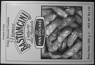
# Box in a scene — matching target
urllib.request.urlretrieve(
    "https://raw.githubusercontent.com/opencv/opencv/master/samples/data/box_in_scene.png",
    "box_in_scene.png"
)

Box object — used as the query image for feature matching

1. Corner Detection with Harris & Shi-Tomasi

Corners are the simplest type of feature — they're distinctive because the intensity changes in multiple directions.

Harris Corner Detector

import cv2
import numpy as np

img = cv2.imread("box.png")
gray = cv2.cvtColor(img, cv2.COLOR_BGR2GRAY)
gray = np.float32(gray)

# blockSize=2, ksize=3 (Sobel kernel), k=0.04 (Harris free parameter)
harris = cv2.cornerHarris(gray, blockSize=2, ksize=3, k=0.04)

# Dilate to mark corners more visibly
harris = cv2.dilate(harris, None)

# Threshold and mark corners in red
output = img.copy()
output[harris > 0.01 * harris.max()] = [0, 0, 255]

cv2.imshow("Harris Corners", output)
cv2.waitKey(0)
cv2.destroyAllWindows()

Shi-Tomasi (Good Features to Track)

Shi-Tomasi is generally more stable than Harris and is the default corner detector used in optical flow:

import cv2

img = cv2.imread("building.jpg")
gray = cv2.cvtColor(img, cv2.COLOR_BGR2GRAY)

# Find up to 100 strongest corners, min quality 0.01, min distance 10px
corners = cv2.goodFeaturesToTrack(gray, maxCorners=100, qualityLevel=0.01, minDistance=10)

output = img.copy()
if corners is not None:
    corners = corners.astype(int)
    for corner in corners:
        x, y = corner.ravel()
        cv2.circle(output, (x, y), 5, (0, 255, 0), -1)

cv2.imshow("Shi-Tomasi Corners", output)
cv2.waitKey(0)
cv2.destroyAllWindows()

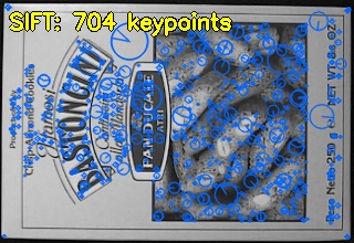
2. SIFT — Scale-Invariant Feature Transform

SIFT detects keypoints that are invariant to scale, rotation, and partially to illumination changes. Each keypoint comes with a 128-dimensional descriptor.

OpenCV 4.x note: SIFT's patent expired in 2020 and it is now part of the main cv2 module — no need for opencv-contrib to use it.

import cv2

img = cv2.imread("building.jpg")
gray = cv2.cvtColor(img, cv2.COLOR_BGR2GRAY)

# Create SIFT detector
sift = cv2.SIFT_create()

# Detect keypoints and compute descriptors
keypoints, descriptors = sift.detectAndCompute(gray, None)
print(f"SIFT found {len(keypoints)} keypoints")

# Draw keypoints
output = cv2.drawKeypoints(
    img, keypoints, None,
    flags=cv2.DRAW_MATCHES_FLAGS_DRAW_RICH_KEYPOINTS
)
cv2.imshow("SIFT Keypoints", output)
cv2.waitKey(0)
cv2.destroyAllWindows()

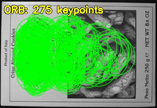
3. ORB — Oriented FAST and Rotated BRIEF

ORB is a fast, open-source alternative to SIFT and SURF. It's rotation-invariant, much faster, and well-suited for real-time applications.

import cv2

img = cv2.imread("building.jpg")
gray = cv2.cvtColor(img, cv2.COLOR_BGR2GRAY)

# Create ORB detector — nfeatures limits the number of keypoints
orb = cv2.ORB_create(nfeatures=500)

keypoints, descriptors = orb.detectAndCompute(gray, None)
print(f"ORB found {len(keypoints)} keypoints")

output = cv2.drawKeypoints(img, keypoints, None, color=(0, 255, 0))
cv2.imshow("ORB Keypoints", output)
cv2.waitKey(0)
cv2.destroyAllWindows()

SIFT vs ORB:

	SIFT	ORB
Speed	Slower	~100x faster
Descriptor	128-dim float	256-bit binary
Scale invariant	Yes	Yes
Rotation invariant	Yes	Yes
License	Free (since 2020)	Free
Best for	Accuracy	Real-time

4. Feature Matching with BFMatcher

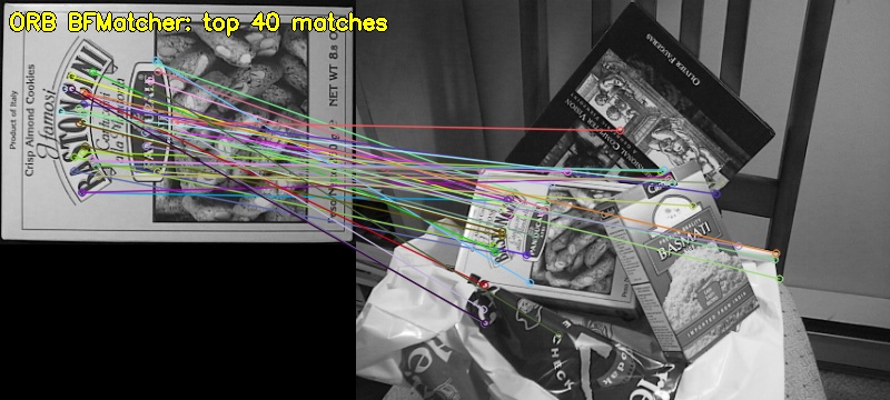
BFMatcher (Brute-Force Matcher) compares every descriptor in one image against every descriptor in the other and returns the best matches.

import cv2

img1 = cv2.imread("box.png", cv2.IMREAD_GRAYSCALE)
img2 = cv2.imread("box_in_scene.png", cv2.IMREAD_GRAYSCALE)

orb = cv2.ORB_create(nfeatures=500)
kp1, des1 = orb.detectAndCompute(img1, None)
kp2, des2 = orb.detectAndCompute(img2, None)

# BFMatcher with Hamming distance (for binary descriptors like ORB)
bf = cv2.BFMatcher(cv2.NORM_HAMMING, crossCheck=True)
matches = bf.match(des1, des2)

# Sort matches by distance (lower = better)
matches = sorted(matches, key=lambda x: x.distance)

# Draw the top 30 matches
result = cv2.drawMatches(img1, kp1, img2, kp2, matches[:30], None,
                         flags=cv2.DrawMatchesFlags_NOT_DRAW_SINGLE_POINTS)
cv2.imshow("ORB Matches", result)
cv2.waitKey(0)
cv2.destroyAllWindows()

5. KNN Matching with Ratio Test (Lowe's Ratio Test)

For SIFT, use knnMatch with David Lowe's ratio test to filter out ambiguous matches:

import cv2

img1 = cv2.imread("box.png", cv2.IMREAD_GRAYSCALE)
img2 = cv2.imread("box_in_scene.png", cv2.IMREAD_GRAYSCALE)

sift = cv2.SIFT_create()
kp1, des1 = sift.detectAndCompute(img1, None)
kp2, des2 = sift.detectAndCompute(img2, None)

# BFMatcher with L2 norm (for float descriptors like SIFT)
bf = cv2.BFMatcher(cv2.NORM_L2)

# Find 2 best matches for each descriptor
matches = bf.knnMatch(des1, des2, k=2)

# Lowe's ratio test — keep matches where the best is significantly better than second best
good_matches = []
for m, n in matches:
    if m.distance < 0.75 * n.distance:
        good_matches.append(m)

print(f"Good matches: {len(good_matches)} / {len(matches)}")

result = cv2.drawMatches(img1, kp1, img2, kp2, good_matches, None,
                         flags=cv2.DrawMatchesFlags_NOT_DRAW_SINGLE_POINTS)
cv2.imshow("SIFT Matches (Ratio Test)", result)
cv2.waitKey(0)
cv2.destroyAllWindows()

6. FLANN-Based Matcher

FLANN (Fast Library for Approximate Nearest Neighbors) is significantly faster than brute force for large descriptor sets:

import cv2

img1 = cv2.imread("box.png", cv2.IMREAD_GRAYSCALE)
img2 = cv2.imread("box_in_scene.png", cv2.IMREAD_GRAYSCALE)

sift = cv2.SIFT_create()
kp1, des1 = sift.detectAndCompute(img1, None)
kp2, des2 = sift.detectAndCompute(img2, None)

# FLANN parameters for SIFT (float descriptors)
FLANN_INDEX_KDTREE = 1
index_params = dict(algorithm=FLANN_INDEX_KDTREE, trees=5)
search_params = dict(checks=50)

flann = cv2.FlannBasedMatcher(index_params, search_params)
matches = flann.knnMatch(des1, des2, k=2)

# Ratio test
good_matches = [m for m, n in matches if m.distance < 0.75 * n.distance]

result = cv2.drawMatchesKnn(img1, kp1, img2, kp2,
                             [[m] for m in good_matches], None,
                             matchColor=(0, 255, 0),
                             singlePointColor=(255, 0, 0),
                             flags=cv2.DrawMatchesFlags_DEFAULT)
cv2.imshow("FLANN Matches", result)
cv2.waitKey(0)
cv2.destroyAllWindows()

7. Homography: Locating an Object in a Scene

With enough good matches, you can compute a homography to find the exact location and pose of an object in a scene:

import cv2
import numpy as np

img_object = cv2.imread("box.png", cv2.IMREAD_GRAYSCALE)
img_scene = cv2.imread("box_in_scene.png", cv2.IMREAD_GRAYSCALE)

sift = cv2.SIFT_create()
kp1, des1 = sift.detectAndCompute(img_object, None)
kp2, des2 = sift.detectAndCompute(img_scene, None)

bf = cv2.BFMatcher(cv2.NORM_L2)
matches = bf.knnMatch(des1, des2, k=2)
good = [m for m, n in matches if m.distance < 0.75 * n.distance]

MIN_MATCH_COUNT = 10
if len(good) >= MIN_MATCH_COUNT:
    src_pts = np.float32([kp1[m.queryIdx].pt for m in good]).reshape(-1, 1, 2)
    dst_pts = np.float32([kp2[m.trainIdx].pt for m in good]).reshape(-1, 1, 2)

    # RANSAC robustly estimates the homography despite outliers
    H, mask = cv2.findHomography(src_pts, dst_pts, cv2.RANSAC, 5.0)

    # Project the object bounding box into the scene
    h, w = img_object.shape
    corners = np.float32([[0, 0], [0, h-1], [w-1, h-1], [w-1, 0]]).reshape(-1, 1, 2)
    transformed = cv2.perspectiveTransform(corners, H)

    # Draw the bounding box on the scene
    scene_color = cv2.cvtColor(img_scene, cv2.COLOR_GRAY2BGR)
    cv2.polylines(scene_color, [np.int32(transformed)], True, (0, 255, 0), 3)
    cv2.imshow("Object Located", scene_color)
else:
    print(f"Not enough matches: {len(good)} / {MIN_MATCH_COUNT}")

cv2.waitKey(0)
cv2.destroyAllWindows()

ORB keypoints detected on the box object (rich keypoint visualization showing scale and orientation)

SIFT keypoints on the same object — more numerous and scale-aware than ORB

ORB BFMatcher: top 40 matches between box (left) and box-in-scene (right)

Conclusion

Feature detection and matching enable image-level understanding that goes far beyond pixel comparisons. ORB is your go-to for real-time applications; SIFT for accuracy-critical work. In the next lesson, we will cover video processing and optical flow — where these techniques come to life in moving scenes.