Lesson 08: Thresholding & Morphological Operations

Thresholding converts a grayscale image into a binary image — separating pixels into foreground and background. Morphological operations then let you clean up, grow, or erode those binary regions. Together, they form the backbone of classical image segmentation.

0. Download the Test Images

This lesson uses two images — a sudoku puzzle (perfect for adaptive thresholding under uneven lighting) and a coins photo (classic morphology demo):

import urllib.request

# Sudoku photo — uneven lighting makes it ideal for adaptive thresholding
urllib.request.urlretrieve(
    "https://raw.githubusercontent.com/opencv/opencv/master/samples/data/sudoku.png",
    "sudoku.png"
)

# Coins on a surface — great for Otsu + morphology to separate touching coins
urllib.request.urlretrieve(
    "https://raw.githubusercontent.com/opencv/opencv/master/samples/data/coins.png",
    "coins.png"
)

Sudoku puzzle with uneven lighting — adaptive thresholding handles this well

1. Simple Thresholding

The most basic form: if a pixel value exceeds a threshold, set it to maxval; otherwise set it to 0 (or vice versa).

import cv2

img = cv2.imread("image.jpg")
gray = cv2.cvtColor(img, cv2.COLOR_BGR2GRAY)

# Binary threshold: pixels > 127 → 255, else 0
ret, binary = cv2.threshold(gray, 127, 255, cv2.THRESH_BINARY)

# Inverse binary: pixels > 127 → 0, else 255
ret, binary_inv = cv2.threshold(gray, 127, 255, cv2.THRESH_BINARY_INV)

# Truncate: pixels > 127 → 127, else unchanged
ret, trunc = cv2.threshold(gray, 127, 255, cv2.THRESH_TRUNC)

cv2.imshow("Binary", binary)
cv2.imshow("Binary Inverse", binary_inv)
cv2.imshow("Truncate", trunc)
cv2.waitKey(0)
cv2.destroyAllWindows()

Threshold types:

Flag	Behavior
`THRESH_BINARY`	`src > thresh → maxval`, else `0`
`THRESH_BINARY_INV`	`src > thresh → 0`, else `maxval`
`THRESH_TRUNC`	`src > thresh → thresh`, else unchanged
`THRESH_TOZERO`	`src > thresh → src`, else `0`
`THRESH_TOZERO_INV`	`src > thresh → 0`, else `src`

2. Otsu's Thresholding

Choosing the threshold manually is error-prone. Otsu's method automatically finds the optimal threshold that minimizes intra-class variance — it works best when the image histogram is bimodal (two distinct peaks).

import cv2

img = cv2.imread("image.jpg")
gray = cv2.cvtColor(img, cv2.COLOR_BGR2GRAY)

# Otsu's threshold — pass 0 as threshold value, OpenCV computes it
otsu_val, binary_otsu = cv2.threshold(
    gray, 0, 255, cv2.THRESH_BINARY + cv2.THRESH_OTSU
)
print(f"Otsu threshold: {otsu_val}")

cv2.imshow("Otsu Binary", binary_otsu)
cv2.waitKey(0)
cv2.destroyAllWindows()

OpenCV 4.x note: The cv2.threshold() function now returns the computed threshold value as the first return value even when using Otsu — useful for debugging or reusing the threshold elsewhere.

3. Adaptive Thresholding

Simple thresholding struggles with non-uniform lighting. Adaptive thresholding computes a local threshold for each pixel based on its neighborhood.

import cv2

img = cv2.imread("image.jpg")
gray = cv2.cvtColor(img, cv2.COLOR_BGR2GRAY)

# Mean adaptive threshold — threshold is mean of neighborhood
adaptive_mean = cv2.adaptiveThreshold(
    gray, 255,
    cv2.ADAPTIVE_THRESH_MEAN_C,
    cv2.THRESH_BINARY,
    blockSize=11,   # neighborhood size (must be odd)
    C=2             # constant subtracted from mean
)

# Gaussian adaptive threshold — threshold is Gaussian-weighted sum of neighborhood
adaptive_gauss = cv2.adaptiveThreshold(
    gray, 255,
    cv2.ADAPTIVE_THRESH_GAUSSIAN_C,
    cv2.THRESH_BINARY,
    blockSize=11,
    C=2
)

cv2.imshow("Adaptive Mean", adaptive_mean)
cv2.imshow("Adaptive Gaussian", adaptive_gauss)
cv2.waitKey(0)
cv2.destroyAllWindows()

When to use each:

Otsu — uniform lighting, clear foreground/background separation
Adaptive (Mean/Gaussian) — uneven lighting, shadows, document scanning

4. Morphological Operations

Morphological operations process binary (or grayscale) images based on a structuring element (kernel). They are used to remove noise, fill holes, or separate connected objects.

Structuring Elements

import cv2
import numpy as np

# Rectangular kernel 5x5
rect_kernel = cv2.getStructuringElement(cv2.MORPH_RECT, (5, 5))

# Elliptical kernel 5x5
ellipse_kernel = cv2.getStructuringElement(cv2.MORPH_ELLIPSE, (5, 5))

# Cross-shaped kernel 5x5
cross_kernel = cv2.getStructuringElement(cv2.MORPH_CROSS, (5, 5))

Erosion

Erosion shrinks foreground regions — useful for removing small noise pixels.

import cv2
import numpy as np

binary = cv2.imread("binary_image.png", cv2.IMREAD_GRAYSCALE)
kernel = cv2.getStructuringElement(cv2.MORPH_RECT, (5, 5))

eroded = cv2.erode(binary, kernel, iterations=1)

cv2.imshow("Original", binary)
cv2.imshow("Eroded", eroded)
cv2.waitKey(0)
cv2.destroyAllWindows()

Dilation

Dilation expands foreground regions — useful for filling small holes and connecting nearby components.

import cv2
import numpy as np

binary = cv2.imread("binary_image.png", cv2.IMREAD_GRAYSCALE)
kernel = cv2.getStructuringElement(cv2.MORPH_RECT, (5, 5))

dilated = cv2.dilate(binary, kernel, iterations=1)

cv2.imshow("Original", binary)
cv2.imshow("Dilated", dilated)
cv2.waitKey(0)
cv2.destroyAllWindows()

Opening and Closing

Operation	What it does	Use case
Opening (erode then dilate)	Removes small noise pixels	Clean up noisy binary masks
Closing (dilate then erode)	Fills small holes inside regions	Fill gaps in detected objects

import cv2
import numpy as np

binary = cv2.imread("binary_image.png", cv2.IMREAD_GRAYSCALE)
kernel = cv2.getStructuringElement(cv2.MORPH_ELLIPSE, (7, 7))

# Opening: removes small noise
opened = cv2.morphologyEx(binary, cv2.MORPH_OPEN, kernel)

# Closing: fills small holes
closed = cv2.morphologyEx(binary, cv2.MORPH_CLOSE, kernel)

cv2.imshow("Original", binary)
cv2.imshow("Opened", opened)
cv2.imshow("Closed", closed)
cv2.waitKey(0)
cv2.destroyAllWindows()

Morphological Gradient and Top Hat

import cv2
import numpy as np

binary = cv2.imread("binary_image.png", cv2.IMREAD_GRAYSCALE)
kernel = cv2.getStructuringElement(cv2.MORPH_RECT, (5, 5))

# Gradient: difference between dilation and erosion → outlines
gradient = cv2.morphologyEx(binary, cv2.MORPH_GRADIENT, kernel)

# Top hat: difference between original and opening → bright spots on dark background
tophat = cv2.morphologyEx(binary, cv2.MORPH_TOPHAT, kernel)

# Black hat: difference between closing and original → dark spots on bright background
blackhat = cv2.morphologyEx(binary, cv2.MORPH_BLACKHAT, kernel)

5. Practical Example: Reading a Sudoku Grid

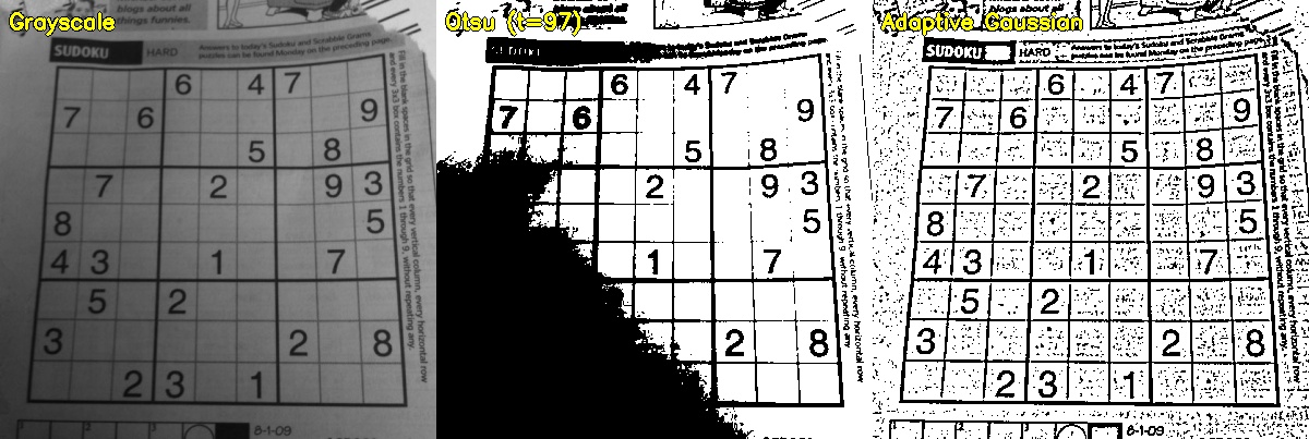
Sudoku photos are a classic thresholding challenge — the lighting is uneven, so simple thresholding fails but adaptive thresholding works perfectly:

import cv2
import numpy as np

img = cv2.imread("sudoku.png")
gray = cv2.cvtColor(img, cv2.COLOR_BGR2GRAY)

# Simple Otsu — fails on uneven lighting
_, otsu = cv2.threshold(gray, 0, 255, cv2.THRESH_BINARY + cv2.THRESH_OTSU)

# Adaptive Gaussian — handles the shadow across the page
adaptive = cv2.adaptiveThreshold(
    gray, 255, cv2.ADAPTIVE_THRESH_GAUSSIAN_C,
    cv2.THRESH_BINARY, blockSize=11, C=2
)

# Show comparison
comparison = cv2.hconcat([
    cv2.cvtColor(gray,     cv2.COLOR_GRAY2BGR),
    cv2.cvtColor(otsu,     cv2.COLOR_GRAY2BGR),
    cv2.cvtColor(adaptive, cv2.COLOR_GRAY2BGR),
])
cv2.imshow("Grayscale | Otsu | Adaptive Gaussian", comparison)
cv2.waitKey(0)
cv2.destroyAllWindows()

# Expected:
# - Otsu: cells in the shadowed area become solid black (too dark threshold)
# - Adaptive: clean grid lines and digits across the entire image

6. Practical Example: Separating Touching Coins

Coins that touch each other in a photo are a morphology classic — erosion separates them, watershed (advanced) counts them:

import cv2
import numpy as np

img = cv2.imread("coins.png")
gray = cv2.cvtColor(img, cv2.COLOR_BGR2GRAY)
blurred = cv2.GaussianBlur(gray, (7, 7), 0)

# Otsu — good here because coins are light on dark background with even lighting
_, binary = cv2.threshold(blurred, 0, 255, cv2.THRESH_BINARY + cv2.THRESH_OTSU)

kernel = cv2.getStructuringElement(cv2.MORPH_ELLIPSE, (5, 5))

# Opening removes small noise specks
opened = cv2.morphologyEx(binary, cv2.MORPH_OPEN, kernel, iterations=2)

# Dilation expands coin regions to fill small holes
sure_bg = cv2.dilate(opened, kernel, iterations=3)

# Erode aggressively to find definite coin centers
sure_fg = cv2.erode(opened, kernel, iterations=4)

# Morphological gradient shows coin outlines
gradient = cv2.morphologyEx(binary, cv2.MORPH_GRADIENT, kernel)

row = cv2.hconcat([
    cv2.cvtColor(binary,   cv2.COLOR_GRAY2BGR),
    cv2.cvtColor(opened,   cv2.COLOR_GRAY2BGR),
    cv2.cvtColor(gradient, cv2.COLOR_GRAY2BGR),
])
cv2.imshow("Binary | Opened | Gradient (outlines)", row)
cv2.waitKey(0)
cv2.destroyAllWindows()

# Expected:
# - Binary: white coin blobs, some touching at edges
# - Opened: same but tiny noise specs removed
# - Gradient: thin white outlines around each coin boundary only

Thresholding comparison: Sudoku — grayscale vs Otsu vs adaptive Gaussian

Morphological operations on coins: binary → opened (noise removed) → closed (gaps filled) → gradient (edges only)

Conclusion

Thresholding separates what you care about from the background; morphological operations refine that separation. In the next lesson, we'll find the actual shapes in those binary masks using contour analysis.