Lesson 11: Video Processing & Optical Flow

Video is just a sequence of image frames. OpenCV makes it easy to read frames from a camera or file, process each one, and write the result back. This lesson also covers optical flow — the apparent motion of pixels between frames — and background subtraction for detecting moving objects.

0. Download a Test Video

We use a freely licensed short traffic clip from the OpenCV test data repository:

import urllib.request

# Short traffic video from OpenCV test assets (~3 MB, 50 frames)
urllib.request.urlretrieve(
    "https://raw.githubusercontent.com/opencv/opencv_extra/master/testdata/cv/video/768x576.avi",
    "traffic.avi"
)
print("Downloaded traffic.avi")

If you prefer to test with your webcam, replace "traffic.avi" with 0 (device index) in any cv2.VideoCapture() call throughout this lesson.

No video file? All examples also work with a live webcam — just swap cv2.VideoCapture("traffic.avi") for cv2.VideoCapture(0).

1. Reading Video

import cv2

# Open a video file
cap = cv2.VideoCapture("traffic.avi")

# Or open the default webcam (device index 0)
# cap = cv2.VideoCapture(0)

if not cap.isOpened():
    print("Error: could not open video")
    exit()

# Read useful properties
fps = cap.get(cv2.CAP_PROP_FPS)
width = int(cap.get(cv2.CAP_PROP_FRAME_WIDTH))
height = int(cap.get(cv2.CAP_PROP_FRAME_HEIGHT))
total_frames = int(cap.get(cv2.CAP_PROP_FRAME_COUNT))
print(f"{width}x{height} @ {fps:.1f} fps, {total_frames} frames")

while True:
    ret, frame = cap.read()
    if not ret:
        break  # End of video

    cv2.imshow("Video", frame)
    if cv2.waitKey(1) & 0xFF == ord("q"):
        break

cap.release()
cv2.destroyAllWindows()

Key VideoCapture properties:

Property	Constant
Frame width	`cv2.CAP_PROP_FRAME_WIDTH`
Frame height	`cv2.CAP_PROP_FRAME_HEIGHT`
FPS	`cv2.CAP_PROP_FPS`
Total frames	`cv2.CAP_PROP_FRAME_COUNT`
Current position (ms)	`cv2.CAP_PROP_POS_MSEC`

OpenCV 4.x note: On Linux, you can pass a GStreamer pipeline string to VideoCapture for hardware-accelerated decoding — e.g., for Jetson Nano: cv2.VideoCapture("v4l2src device=/dev/video0 ! ...").

2. Writing Video

import cv2

cap = cv2.VideoCapture("traffic.avi")
fps = cap.get(cv2.CAP_PROP_FPS)
width = int(cap.get(cv2.CAP_PROP_FRAME_WIDTH))
height = int(cap.get(cv2.CAP_PROP_FRAME_HEIGHT))

# Define codec and create VideoWriter
# Common codecs: 'mp4v' (MP4), 'XVID' (AVI), 'MJPG' (AVI)
fourcc = cv2.VideoWriter_fourcc(*"mp4v")
out = cv2.VideoWriter("output.mp4", fourcc, fps, (width, height))

while True:
    ret, frame = cap.read()
    if not ret:
        break

    # Process frame
    gray = cv2.cvtColor(frame, cv2.COLOR_BGR2GRAY)
    gray_bgr = cv2.cvtColor(gray, cv2.COLOR_GRAY2BGR)  # Writer needs BGR

    out.write(gray_bgr)

cap.release()
out.release()
print("Done writing output.mp4")

3. Background Subtraction

Background subtraction isolates moving objects by comparing each frame to a learned background model. OpenCV provides two high-quality algorithms.

MOG2 (Mixture of Gaussians)

MOG2 models each pixel as a mixture of Gaussians and adapts to slow lighting changes:

import cv2

cap = cv2.VideoCapture("traffic.avi")

# Create background subtractor
# history: number of frames used to build the model
# varThreshold: sensitivity (lower = more sensitive)
# detectShadows: whether to detect and mark shadows
bg_subtractor = cv2.createBackgroundSubtractorMOG2(
    history=500, varThreshold=50, detectShadows=True
)

while True:
    ret, frame = cap.read()
    if not ret:
        break

    # Apply background subtraction
    fg_mask = bg_subtractor.apply(frame)

    # Shadows are marked as 127 — remove them
    _, fg_mask = cv2.threshold(fg_mask, 200, 255, cv2.THRESH_BINARY)

    # Clean up the mask
    kernel = cv2.getStructuringElement(cv2.MORPH_ELLIPSE, (5, 5))
    fg_mask = cv2.morphologyEx(fg_mask, cv2.MORPH_OPEN, kernel)

    cv2.imshow("Frame", frame)
    cv2.imshow("Foreground Mask", fg_mask)
    if cv2.waitKey(30) & 0xFF == ord("q"):
        break

cap.release()
cv2.destroyAllWindows()

KNN Background Subtractor

KNN is more accurate at detecting slow-moving or stationary foreground objects:

import cv2

cap = cv2.VideoCapture("traffic.avi")
bg_subtractor = cv2.createBackgroundSubtractorKNN(
    history=500, dist2Threshold=400, detectShadows=True
)

while True:
    ret, frame = cap.read()
    if not ret:
        break

    fg_mask = bg_subtractor.apply(frame)
    cv2.imshow("KNN Foreground", fg_mask)
    if cv2.waitKey(30) & 0xFF == ord("q"):
        break

cap.release()
cv2.destroyAllWindows()

4. Optical Flow

Optical flow computes the motion of pixels between consecutive frames.

Lucas-Kanade Sparse Optical Flow

Tracks a sparse set of keypoints from frame to frame — fast and suitable for real-time tracking:

import cv2
import numpy as np

cap = cv2.VideoCapture("traffic.avi")
ret, old_frame = cap.read()
old_gray = cv2.cvtColor(old_frame, cv2.COLOR_BGR2GRAY)

# Detect initial keypoints to track
feature_params = dict(maxCorners=200, qualityLevel=0.3, minDistance=7, blockSize=7)
p0 = cv2.goodFeaturesToTrack(old_gray, mask=None, **feature_params)

# Parameters for Lucas-Kanade optical flow
lk_params = dict(
    winSize=(15, 15),
    maxLevel=2,
    criteria=(cv2.TERM_CRITERIA_EPS | cv2.TERM_CRITERIA_COUNT, 10, 0.03)
)

# Mask for drawing trails
mask = np.zeros_like(old_frame)
colors = np.random.randint(0, 255, (200, 3))

while True:
    ret, frame = cap.read()
    if not ret or p0 is None:
        break
    frame_gray = cv2.cvtColor(frame, cv2.COLOR_BGR2GRAY)

    # Calculate optical flow — track p0 in the new frame
    p1, status, _ = cv2.calcOpticalFlowPyrLK(old_gray, frame_gray, p0, None, **lk_params)

    # Select good points (status == 1 means successfully tracked)
    if p1 is not None:
        good_new = p1[status == 1]
        good_old = p0[status == 1]

        # Draw motion trails
        for i, (new, old) in enumerate(zip(good_new, good_old)):
            a, b = new.ravel().astype(int)
            c, d = old.ravel().astype(int)
            mask = cv2.line(mask, (a, b), (c, d), colors[i % 200].tolist(), 2)
            frame = cv2.circle(frame, (a, b), 4, colors[i % 200].tolist(), -1)

        output = cv2.add(frame, mask)
        cv2.imshow("Sparse Optical Flow", output)
        old_gray = frame_gray.copy()
        p0 = good_new.reshape(-1, 1, 2)

    if cv2.waitKey(30) & 0xFF == ord("q"):
        break

cap.release()
cv2.destroyAllWindows()

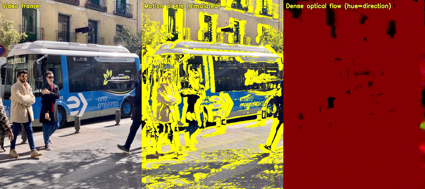
Farneback Dense Optical Flow

Computes flow for every pixel — more information but slower:

import cv2
import numpy as np

cap = cv2.VideoCapture("traffic.avi")
ret, frame1 = cap.read()
prev_gray = cv2.cvtColor(frame1, cv2.COLOR_BGR2GRAY)

# HSV image for visualization
hsv = np.zeros_like(frame1)
hsv[..., 1] = 255  # Full saturation

while True:
    ret, frame2 = cap.read()
    if not ret:
        break
    curr_gray = cv2.cvtColor(frame2, cv2.COLOR_BGR2GRAY)

    # Compute dense optical flow
    flow = cv2.calcOpticalFlowFarneback(
        prev_gray, curr_gray,
        None,
        pyr_scale=0.5,   # image scale per pyramid level
        levels=3,         # number of pyramid levels
        winsize=15,       # averaging window size
        iterations=3,     # iterations at each level
        poly_n=5,         # pixel neighborhood size
        poly_sigma=1.2,   # std dev for Gaussian smoothing
        flags=0
    )

    # Convert flow to polar (magnitude + angle) for HSV visualization
    magnitude, angle = cv2.cartToPolar(flow[..., 0], flow[..., 1])
    hsv[..., 0] = angle * 180 / np.pi / 2   # Hue encodes direction
    hsv[..., 2] = cv2.normalize(magnitude, None, 0, 255, cv2.NORM_MINMAX)
    bgr_flow = cv2.cvtColor(hsv, cv2.COLOR_HSV2BGR)

    cv2.imshow("Dense Optical Flow", bgr_flow)
    prev_gray = curr_gray

    if cv2.waitKey(30) & 0xFF == ord("q"):
        break

cap.release()
cv2.destroyAllWindows()

5. Practical Example: Motion Detection System

Combining background subtraction with contour detection to alert on movement:

import cv2
import numpy as np

cap = cv2.VideoCapture(0)  # Webcam
bg_sub = cv2.createBackgroundSubtractorMOG2(history=500, varThreshold=50)
kernel = cv2.getStructuringElement(cv2.MORPH_ELLIPSE, (5, 5))
MIN_AREA = 1500  # Ignore small movements

while True:
    ret, frame = cap.read()
    if not ret:
        break

    fg_mask = bg_sub.apply(frame)
    _, fg_mask = cv2.threshold(fg_mask, 200, 255, cv2.THRESH_BINARY)
    fg_mask = cv2.morphologyEx(fg_mask, cv2.MORPH_OPEN, kernel, iterations=2)
    fg_mask = cv2.dilate(fg_mask, kernel, iterations=2)

    contours, _ = cv2.findContours(fg_mask, cv2.RETR_EXTERNAL, cv2.CHAIN_APPROX_SIMPLE)

    motion_detected = False
    for cnt in contours:
        if cv2.contourArea(cnt) > MIN_AREA:
            motion_detected = True
            x, y, w, h = cv2.boundingRect(cnt)
            cv2.rectangle(frame, (x, y), (x + w, y + h), (0, 255, 0), 2)

    label = "MOTION DETECTED" if motion_detected else "No motion"
    color = (0, 0, 255) if motion_detected else (0, 255, 0)
    cv2.putText(frame, label, (10, 30), cv2.FONT_HERSHEY_SIMPLEX, 1.0, color, 2)

    cv2.imshow("Motion Detection", frame)
    if cv2.waitKey(30) & 0xFF == ord("q"):
        break

cap.release()
cv2.destroyAllWindows()

Video processing visualization: a frame, simulated motion mask (highlighted moving pixels), and dense optical flow (hue encodes direction)

Conclusion

Video processing opens up a whole new dimension in computer vision — time. Background subtraction and optical flow let you understand what's moving and where. In the next lesson, we'll move into deep learning with OpenCV's DNN module, which lets you run modern neural networks entirely within OpenCV.