
Lesson 05: Color Spaces
 Viet-Anh Nguyen
In computer vision, color is an important aspect of images. Understanding how color is represented and manipulated is essential for image processing tasks. In this lesson, we will discuss the different color spaces that are used in computer vision and how to convert between them.
0. Download the Test Image
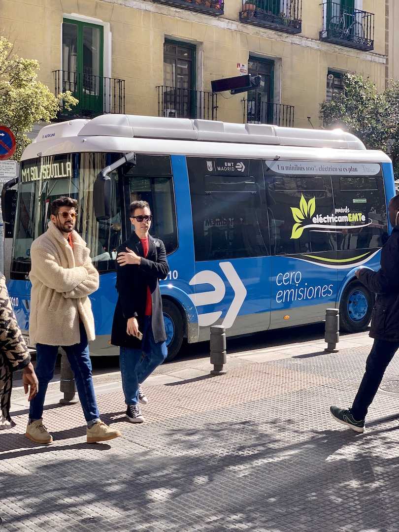
All examples use a colorful street scene. Download it once:
import urllib.request
import cv2

urllib.request.urlretrieve(
    "https://ultralytics.com/images/bus.jpg", "bus.jpg"
)
1. Color Spaces
A color space is a mathematical representation of a set of colors. There are many different color spaces, but the most commonly used ones in computer vision are RGB, HSV, and Grayscale.
a. RGB Color Space
RGB stands for Red, Green, Blue. In the RGB color space, each color is represented by a combination of three primary colors: red, green, and blue. The values for each color channel range from 0 to 255. For example, the color red is represented by the values (255, 0, 0), while the color green is represented by the values (0, 255, 0).
import cv2

# Read an image
img = cv2.imread("bus.jpg")

# Convert the image to the RGB color space
rgb_img = cv2.cvtColor(img, cv2.COLOR_BGR2RGB)

# Display the image
cv2.imshow("Image", rgb_img)
b. HSV Color Space
HSV stands for Hue, Saturation, Value. The HSV color space separates color information into three components: hue, saturation, and value. The hue component represents the color itself, the saturation component represents the purity of the color, and the value component represents the brightness of the color.
import cv2

# Read an image
img = cv2.imread("bus.jpg")

# Convert the image to the HSV color space
hsv_img = cv2.cvtColor(img, cv2.COLOR_BGR2HSV)

# Display the image
cv2.imshow("Image", hsv_img)
c. Grayscale Color Space
Grayscale is a single-channel color space that represents images using shades of gray. In the grayscale color space, each pixel is represented by a single value ranging from 0 (black) to 255 (white).
import cv2

# Read an image
img = cv2.imread("bus.jpg")

# Convert the image to the grayscale color space
gray_img = cv2.cvtColor(img, cv2.COLOR_BGR2GRAY)

# Display the image
cv2.imshow("Image", gray_img)
d. Color Space Conversion
OpenCV provides a convenient way to convert between color spaces using the cv2.cvtColor() function. This function takes the image data and the color space conversion code as its input.
import cv2

# Read an image
img = cv2.imread("bus.jpg")

# Convert the image to the HSV color space
hsv_img = cv2.cvtColor(img, cv2.COLOR_BGR2HSV)

# Convert the image to the grayscale color space
gray_img = cv2.cvtColor(img, cv2.COLOR_BGR2GRAY)
2. Applications
Color spaces are used in many computer vision applications, such as object detection and image segmentation. For example, in object detection, the HSV color space can be used to identify specific colors in an image, while in image segmentation, the grayscale color space can be used to separate the foreground from the background. Here are some examples of applications of color spaces in OpenCV with example code:
a. Object Detection using HSV Color Space
The HSV color space can be used to identify specific colors in an image, making it useful for object detection. In this example, we will detect red objects in an image.
import cv2
import numpy as np

# Read an image
img = cv2.imread("bus.jpg")

# Convert the image to the HSV color space
hsv_img = cv2.cvtColor(img, cv2.COLOR_BGR2HSV)

# Define the range of red color in HSV
lower_red = np.array([0, 50, 50])
upper_red = np.array([10, 255, 255])
mask1 = cv2.inRange(hsv_img, lower_red, upper_red)

lower_red = np.array([170, 50, 50])
upper_red = np.array([180, 255, 255])
mask2 = cv2.inRange(hsv_img, lower_red, upper_red)

# Combine the two masks
mask = cv2.bitwise_or(mask1, mask2)

# Apply the mask to the original image
res = cv2.bitwise_and(img, img, mask=mask)

# Show the result
cv2.imshow("Image", img)
cv2.imshow("Mask", mask)
cv2.imshow("Result", res)
cv2.waitKey(0)
cv2.destroyAllWindows()
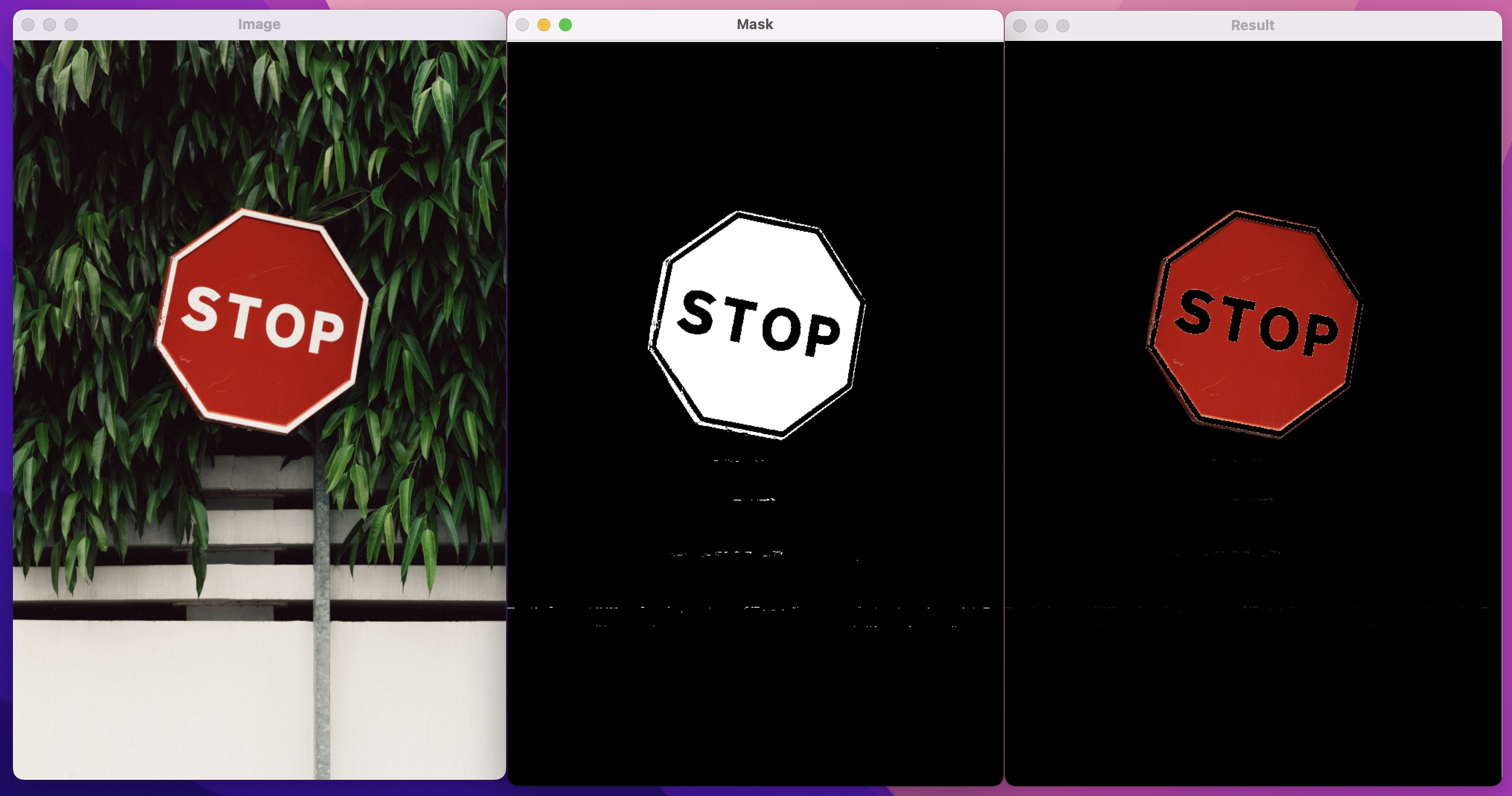
The first step is to read an image using the cv2.imread() function and store it in the img variable.
Next, the image is converted from the BGR color space to the HSV color space using the cv2.cvtColor() function. The resulting image is stored in the hsv_img variable.
To extract the red-colored objects from the image, we need to define the range of red color in the HSV color space. This is done by defining two arrays lower_red and upper_red, which represent the lower and upper bounds of the red color, respectively.
In the HSV color space, the hue (H) ranges from 0 to 179. However, the red color wraps around the spectrum, so it can be found in two different ranges: 0-10 and 170-180. Therefore, we need to define two ranges to include the entire range of red color. In this example, we define lower_red and upper_red twice for each range of red.
Then, we use the cv2.inRange() function to create two masks for each range of red. The cv2.inRange() function returns a binary mask that represents the pixels within the specified color range.
Next, we combine the two masks using the cv2.bitwise_or() function to obtain a single mask that includes all the red-colored objects in the image.
Finally, we apply the mask to the original image using the cv2.bitwise_and() function to extract the red-colored objects. The resulting image is stored in the res variable.
To display the result, we use the cv2.imshow() function to create a window with the resulting image and the cv2.waitKey() function to wait for a key press before closing the window. The cv2.destroyAllWindows() function is used to close all windows created by OpenCV.
b. Image Segmentation using Grayscale Color Space
The grayscale color space can be used for image segmentation, where we separate the foreground from the background. In this example, we will segment a grayscale image using Otsu's thresholding.
import cv2

# Read a grayscale image
img = cv2.imread("path/to/image.jpg", cv2.IMREAD_GRAYSCALE)

# Apply Otsu's thresholding
_, thresh = cv2.threshold(img, 0, 255, cv2.THRESH_BINARY+cv2.THRESH_OTSU)

# Show the result
cv2.imshow("Image", img)
cv2.imshow("Result", thresh)
cv2.waitKey(0)
cv2.destroyAllWindows()
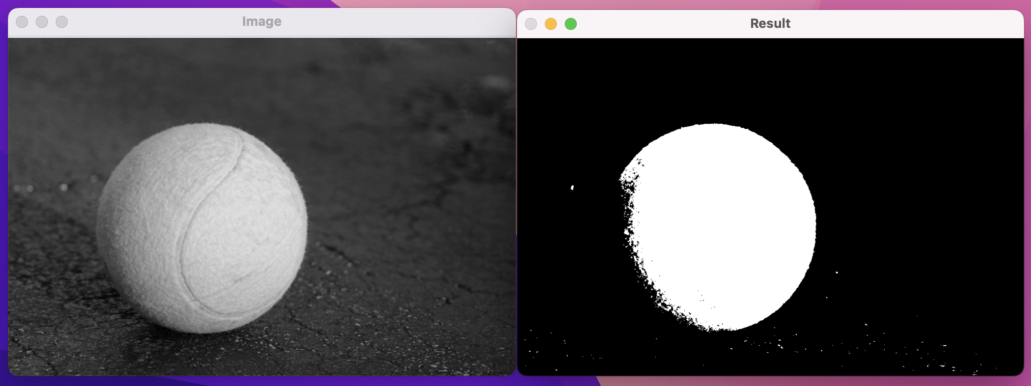
First, an image is read in grayscale using the cv2.imread() function and the cv2.IMREAD_GRAYSCALE flag. The resulting image is stored in the img variable.
Otsu's thresholding is a technique that automatically calculates a threshold value to separate the foreground and background pixels in an image. It works by maximizing the variance between the two groups of pixels. The cv2.threshold() function is used to apply Otsu's thresholding to the grayscale image.
The cv2.threshold() function takes the following arguments:
img: the input imagethresh: the threshold value calculated by the algorithm (this parameter is not used in Otsu's thresholding)maxval: the maximum value to be assigned to pixels that are above the threshold valuetype: the type of thresholding to be applied. In this example, we usecv2.THRESH_BINARY+cv2.THRESH_OTSUto apply Otsu's thresholding and set all pixels above the threshold value to 255.
The cv2.threshold() function returns two values: the threshold value used and the thresholded image. In this example, we only store the thresholded image in the thresh variable.
c. Color Correction using RGB Color Space
The RGB color space can be used for color correction, where we adjust the color balance of an image. In this example, we will adjust the color balance of an image by scaling the values of the red, green, and blue channels.
import cv2

# Read an image
original_img = cv2.imread("bus.jpg")
img = original_img.copy()

# Scale the values of the red, green, and blue channels
img[:, :, 0] = img[:, :, 0] * 0.8  # Red channel
img[:, :, 1] = img[:, :, 1] * 1.05  # Green channel
img[:, :, 2] = img[:, :, 2] * 0.8  # Blue channel

# Show the result
cv2.imshow("Image", original_img)
cv2.imshow("Result", img)
cv2.waitKey(0)
cv2.destroyAllWindows()
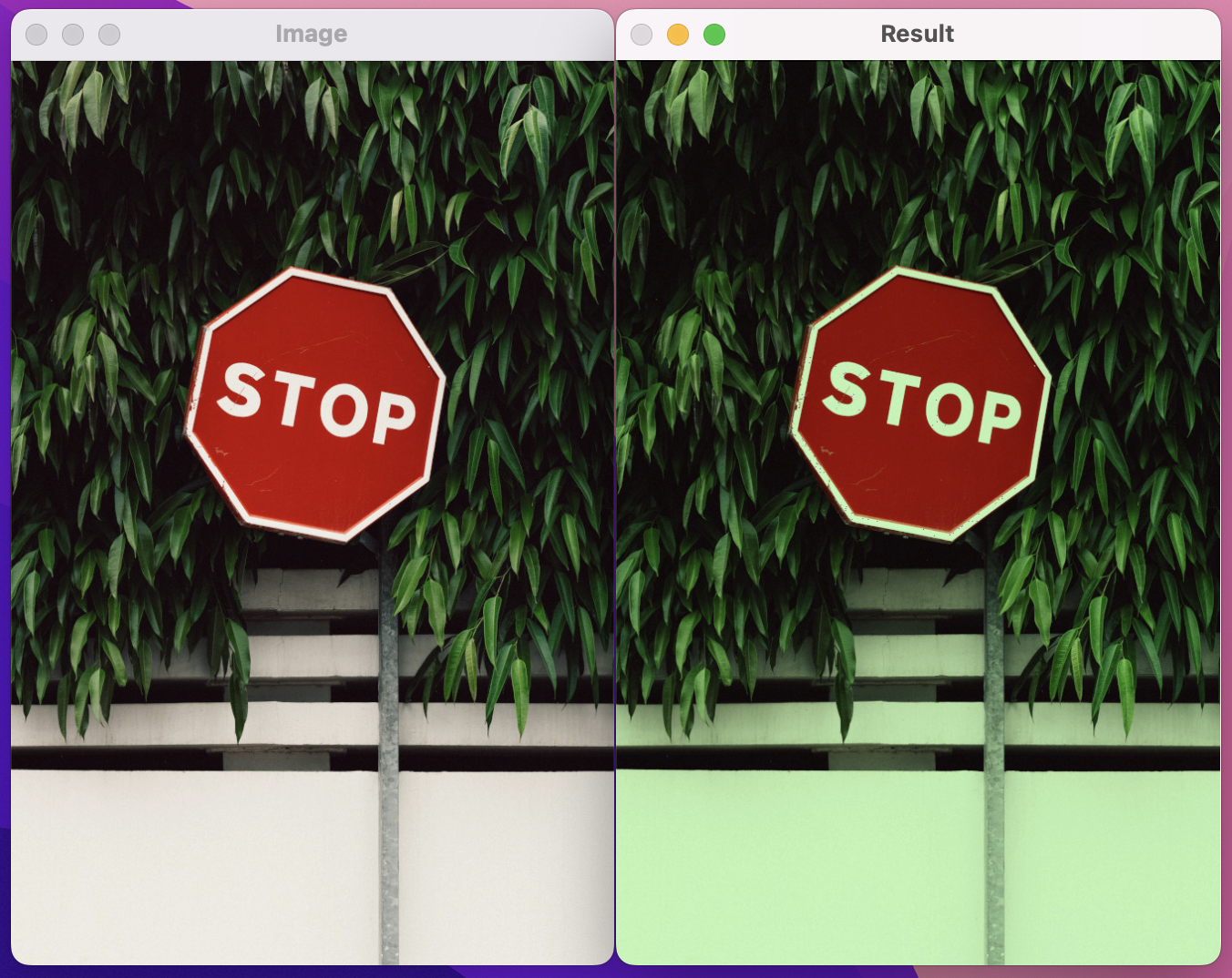
The code scales the values of the red, green, and blue channels of the image by multiplying each channel by a scalar value. The first line of code img[:, :, 0] = img[:, :, 0] * 0.8 scales the values of the red channel by 0.8, the second line of code img[:, :, 1] = img[:, :, 1] * 1.05 scales the values of the green channel by 1.05, and the third line of code img[:, :, 2] = img[:, :, 2] * 0.8 scales the values of the blue channel by 0.8. This will change the overall color balance of the image.
These are just a few examples of the applications of color spaces in OpenCV. There are many more applications, and understanding color spaces is essential for image processing tasks in computer vision.
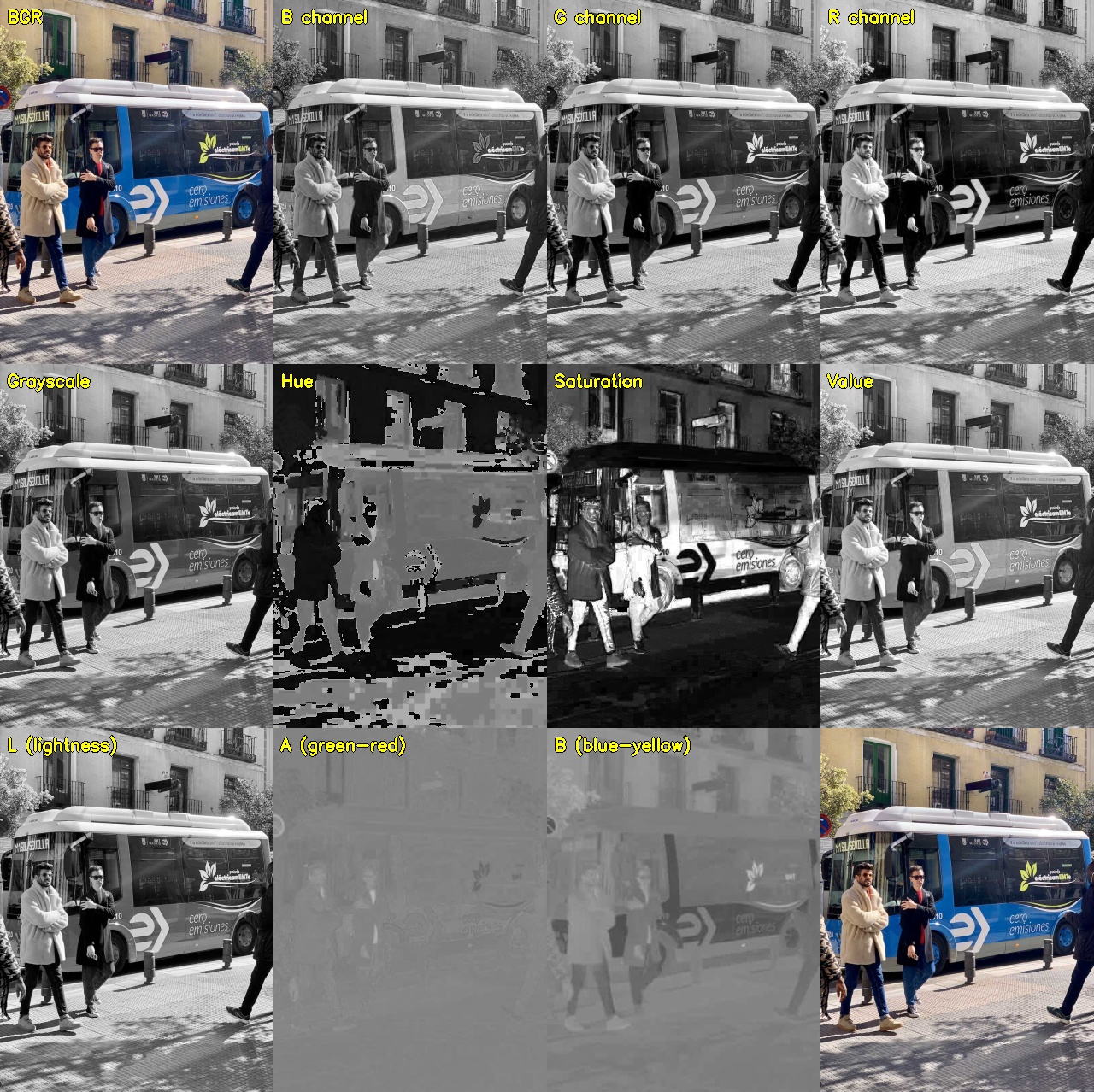
3. Visualizing All Channels Side by Side
Here is a complete script that splits the bus image into all major color space channels and displays them in a grid — great for building intuition about what each channel captures:
import cv2
import numpy as np
import urllib.request

urllib.request.urlretrieve("https://ultralytics.com/images/bus.jpg", "bus.jpg")
img = cv2.imread("bus.jpg")
img = cv2.resize(img, (400, 300))  # shrink for display

hsv = cv2.cvtColor(img, cv2.COLOR_BGR2HSV)
lab = cv2.cvtColor(img, cv2.COLOR_BGR2LAB)

def to_bgr(channel):
    """Convert single-channel to 3-channel for display."""
    return cv2.cvtColor(channel, cv2.COLOR_GRAY2BGR)

row1 = cv2.hconcat([img,              to_bgr(img[:,:,0]),  to_bgr(img[:,:,1]),  to_bgr(img[:,:,2])])
row2 = cv2.hconcat([to_bgr(cv2.cvtColor(img, cv2.COLOR_BGR2GRAY)),
                    to_bgr(hsv[:,:,0]), to_bgr(hsv[:,:,1]), to_bgr(hsv[:,:,2])])
row3 = cv2.hconcat([img,              to_bgr(lab[:,:,0]),  to_bgr(lab[:,:,1]),  to_bgr(lab[:,:,2])])

grid = cv2.vconcat([row1, row2, row3])
cv2.imshow("Channels: BGR | B G R / Gray | H S V / BGR | L A B", grid)
cv2.waitKey(0)
cv2.destroyAllWindows()

# Expected:
# Row 1: full color | blue channel (sky is bright) | green channel | red channel (bus is bright)
# Row 2: grayscale | hue (encodes color type) | saturation (vivid=bright) | value (brightness)
# Row 3: full color | L (lightness) | A (green-red axis) | B (blue-yellow axis)
4. Conclusion
In this lesson, we have discussed the different color spaces that are used in computer vision, how to convert between them, and how they can be used in applications. Understanding color spaces is essential for image processing tasks and can help you achieve better results in your computer vision projects.