Lesson 06: Image Filtering for Image Enhancement

Image filtering is an essential technique in image processing that involves the manipulation of the pixel values of an image to achieve various effects. In this lesson, we will cover some of the most commonly used image filtering techniques in image enhancement, including blurring and sharpening.

0. Download the Test Image

import urllib.request
import cv2

# Download a close-up portrait — good for seeing blur/sharpen effects on fine detail
urllib.request.urlretrieve(
    "https://ultralytics.com/images/zidane.jpg", "zidane.jpg"
)
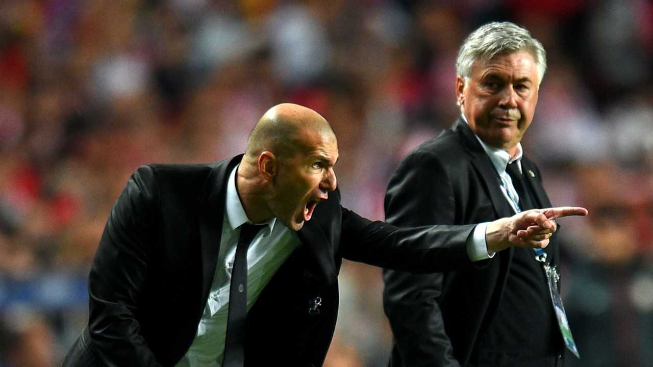
img = cv2.imread("zidane.jpg")
print(f"Loaded: {img.shape}")  # e.g. (720, 1280, 3)

1. Blurring

Blurring is a filtering technique used to reduce the noise in an image. This technique involves convolving the image with a filter kernel that has the effect of averaging the pixel values within a neighborhood. The size of the neighborhood is determined by the size of the filter kernel.

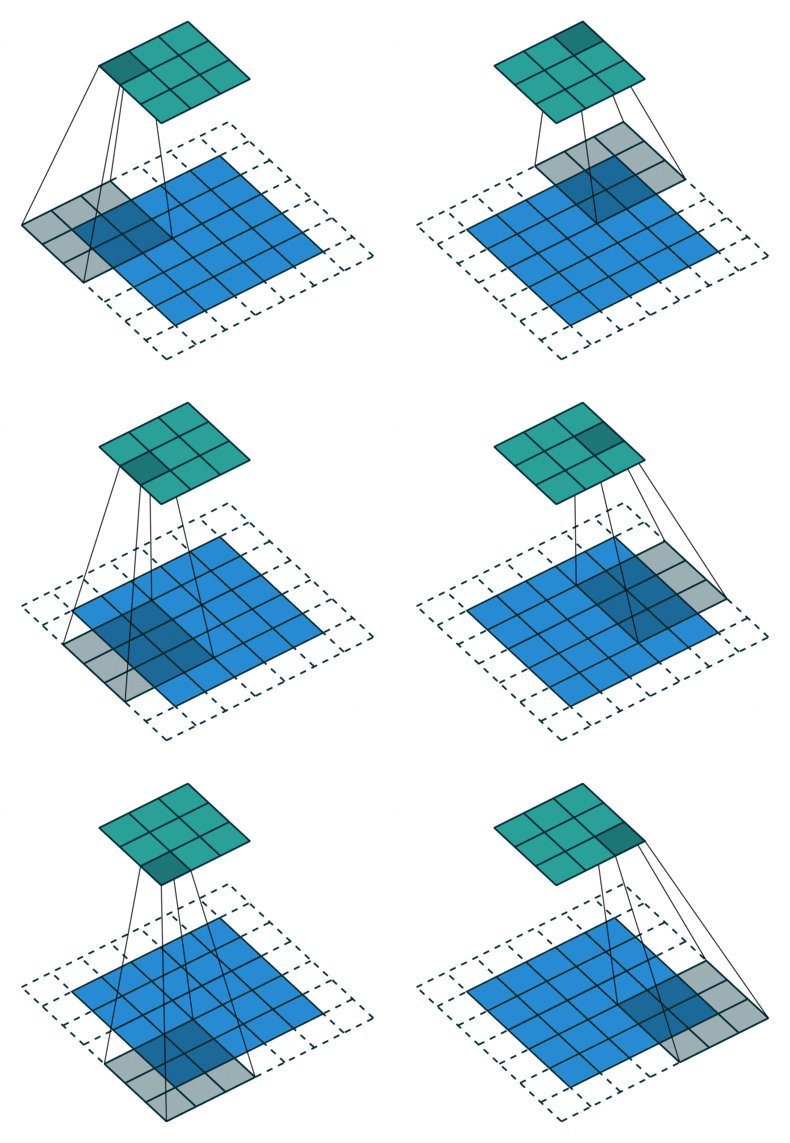
Image convulution - Source: https://github.com/vdumoulin/conv_arithmetic

OpenCV provides several functions for blurring an image, including the cv2.blur(), cv2.GaussianBlur(), cv2.medianBlur(), and cv2.bilateralFilter() functions.

a. Average Blurring

Average blurring is a type of image filtering technique that smooths out an image by replacing the pixel value with the average of the neighboring pixels. This technique can be used to reduce noise in an image or to blur the image for a variety of purposes such as reducing image details or for preprocessing images for further analysis.

The filter kernel used for average blurring is called a box filter, which is a square kernel with equal weights. The size of the kernel determines the size of the neighborhood used for averaging the pixel values.

In OpenCV, we can perform average blurring using the cv2.blur() function. The cv2.blur() function takes two parameters - the input image and the kernel size. The kernel size is a tuple of two integers that specifies the size of the kernel, which is used for averaging the neighboring pixels.

Here is an example of applying average blurring to an image using the cv2.blur() function:

import cv2

# Load the input image
img = cv2.imread("zidane.jpg")

# Apply average blurring with kernel size of (5,5)
blurred_img = cv2.blur(img, (5,5))

# Display the original and blurred images
cv2.imshow("Original Image", img)
cv2.imshow("Blurred Image", blurred_img)
cv2.waitKey(0)
cv2.destroyAllWindows()

In this example, we load an input image using the cv2.imread() function and then apply average blurring to the image using the cv2.blur() function with a kernel size of (5,5). The output image is then displayed using the cv2.imshow() function.

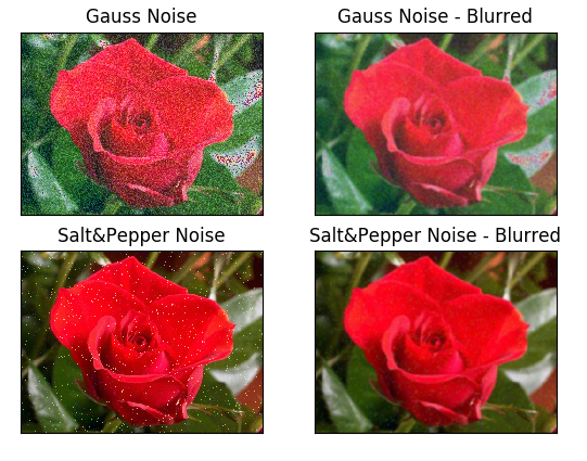
An example of applying average blurring to some noisy images:

b. Gaussian Blurring

Another common blurring technique in computer vision is Gaussian blurring, which is implemented in OpenCV using the cv2.GaussianBlur() function.

Gaussian blurring is similar to average blurring, but instead of a simple box filter, it uses a kernel that follows a Gaussian distribution. The kernel values decrease as the distance from the center increases, resulting in a more natural-looking blur. This technique is particularly useful when preserving edges is important.

The cv2.GaussianBlur() function takes three arguments: the input image, the kernel size (specified as a tuple), and the standard deviation of the Gaussian distribution along the x and y directions. Here"s an example of how to use it:

import cv2

# Read an image
img = cv2.imread("zidane.jpg")

# Apply Gaussian blur with a 5x5 kernel and standard deviation of 0 along x and y directions
blur = cv2.GaussianBlur(img, (5, 5), 0)

# Display the original and blurred images side by side
cv2.imshow("Original", img)
cv2.imshow("Blurred", blur)
cv2.waitKey(0)
cv2.destroyAllWindows()

In this example, we apply Gaussian blur to the input image using a 5x5 kernel and a standard deviation of 0 along the x and y directions. The resulting blurred image is displayed alongside the original for comparison. Note that the amount of blur can be adjusted by changing the kernel size and standard deviation.

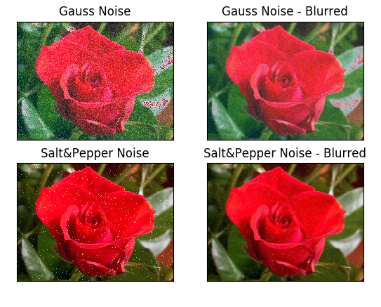
An example of applying Gaussian blurring to some noisy images:

c. Median Blurring

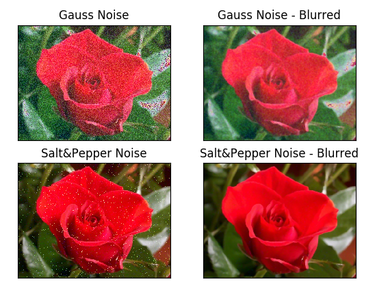
The median filter is another commonly used image filtering technique in computer vision. It is particularly useful for removing salt-and-pepper noise from images. Salt-and-pepper noise is a type of noise that can occur in images, where some pixels are either completely black or completely white.

The median filter works by replacing the pixel value with the median of the neighboring pixel values. This technique is effective at removing salt-and-pepper noise because the median value is less sensitive to outliers than the mean value.

In OpenCV, cv2.medianBlur() function takes two arguments: the input image and the size of the kernel. The kernel size must be a positive odd integer. The function applies a median filter to the image using the specified kernel size.

Here is an example of how to use cv2.medianBlur() to remove salt-and-pepper noise from an image:

import cv2

# Read an image
img = cv2.imread("zidane.jpg")

# Apply median blur with kernel size 5x5
blur_img = cv2.medianBlur(img, 5)

# Show the result
cv2.imshow("Result", blur_img)
cv2.waitKey(0)
cv2.destroyAllWindows()

In this example, we first read an image using cv2.imread(). Then we apply a median blur to the image using a 5x5 kernel size by calling cv2.medianBlur(). Finally, we display the resulting image using cv2.imshow().

Note that the size of the kernel determines the strength of the median filter. A larger kernel size will result in a stronger filter, but may also cause blurring or loss of detail in the image. It is important to choose an appropriate kernel size for the specific image and application.

An example of applying median blurring to some noisy images:

d. Bilateral Filtering

The bilateral filter is another type of image filtering technique that can be used to smooth images while preserving edges. It applies a bilateral filter to the image, which takes into account the intensity differences and spatial distances between pixels.

The bilateral filter is implemented in OpenCV using the cv2.bilateralFilter() function. The syntax is as follows:

cv2.bilateralFilter(src, d, sigmaColor, sigmaSpace[, dst[, borderType]])

• src: the input image.
• d: diameter of each pixel neighborhood used during filtering. Larger values of d will make the image smoother.
• sigmaColor: the standard deviation in the color space. A larger value of sigmaColor means that more colors in the neighborhood will be considered when computing the blur.
• sigmaSpace: the standard deviation in the coordinate space. A larger value of sigmaSpace means that pixels farther away from the center will be considered when computing the blur.
• dst: the output image. If not specified, the function will create an output image with the same size and type as the input image.
• borderType: the type of border to use when applying the filter.

Here"s an example of how to use cv2.bilateralFilter():

import cv2

# Read the input image
img = cv2.imread("zidane.jpg")

# Apply bilateral filtering
bilateral_filtered = cv2.bilateralFilter(img, 9, 75, 75)

# Display the result
cv2.imshow("Bilateral Filtered Image", bilateral_filtered)
cv2.waitKey(0)
cv2.destroyAllWindows()

In this example, d is set to 9, sigmaColor and sigmaSpace are both set to 75. The larger the values of sigmaColor and sigmaSpace, the more smoothing will be applied to the image. The output of cv2.bilateralFilter() will be an image with smoothed edges and reduced noise.

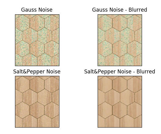
Comparing Gaussian and bilateral filtering: Let"s compare the results of applying Gaussian and bilateral filtering to an image to see the difference between the two techniques.

Result of applying bilateral filtering:

Result of applying Gaussian filtering:

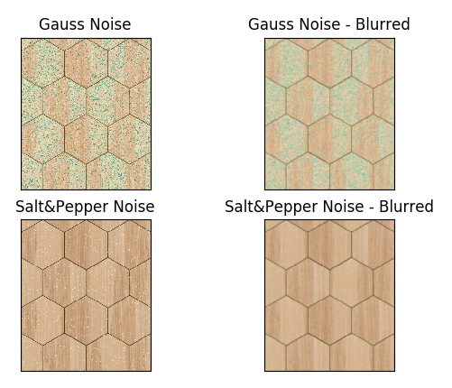
As you can see, the bilateral filter is able to smooth the image while preserving the edges better than the Gaussian filter.

2. Sharpening

Image sharpening is the process of emphasizing the edges in an image to make it appear clearer and more defined. In OpenCV, there are various techniques for image sharpening, such as using a high-pass filter or Laplacian operator. Here, we"ll explore some examples of how to perform image sharpening using OpenCV.

a. High-pass Filtering

One of the most common techniques for image sharpening is to use a high-pass filter. This filter works by amplifying the high-frequency components of an image, such as the edges, while suppressing the low-frequency components, such as the flat regions. In OpenCV, we can use the cv2.filter2D() function to perform high-pass filtering.

Here"s an example code that shows how to perform high-pass filtering on an image:

import cv2
import numpy as np

# Read the image
img = cv2.imread("zidane.jpg")

# Define the kernel for high-pass filtering
kernel = np.array([[-1, -1, -1], [-1, 7, -1], [-1, -1, -1]])

# Apply the high-pass filter
sharpened_img = cv2.filter2D(img, -1, kernel)

# Display the result
cv2.imshow("Original Image", img)
cv2.imshow("High-pass Filtering", sharpened_img)
cv2.waitKey(0)
cv2.destroyAllWindows()

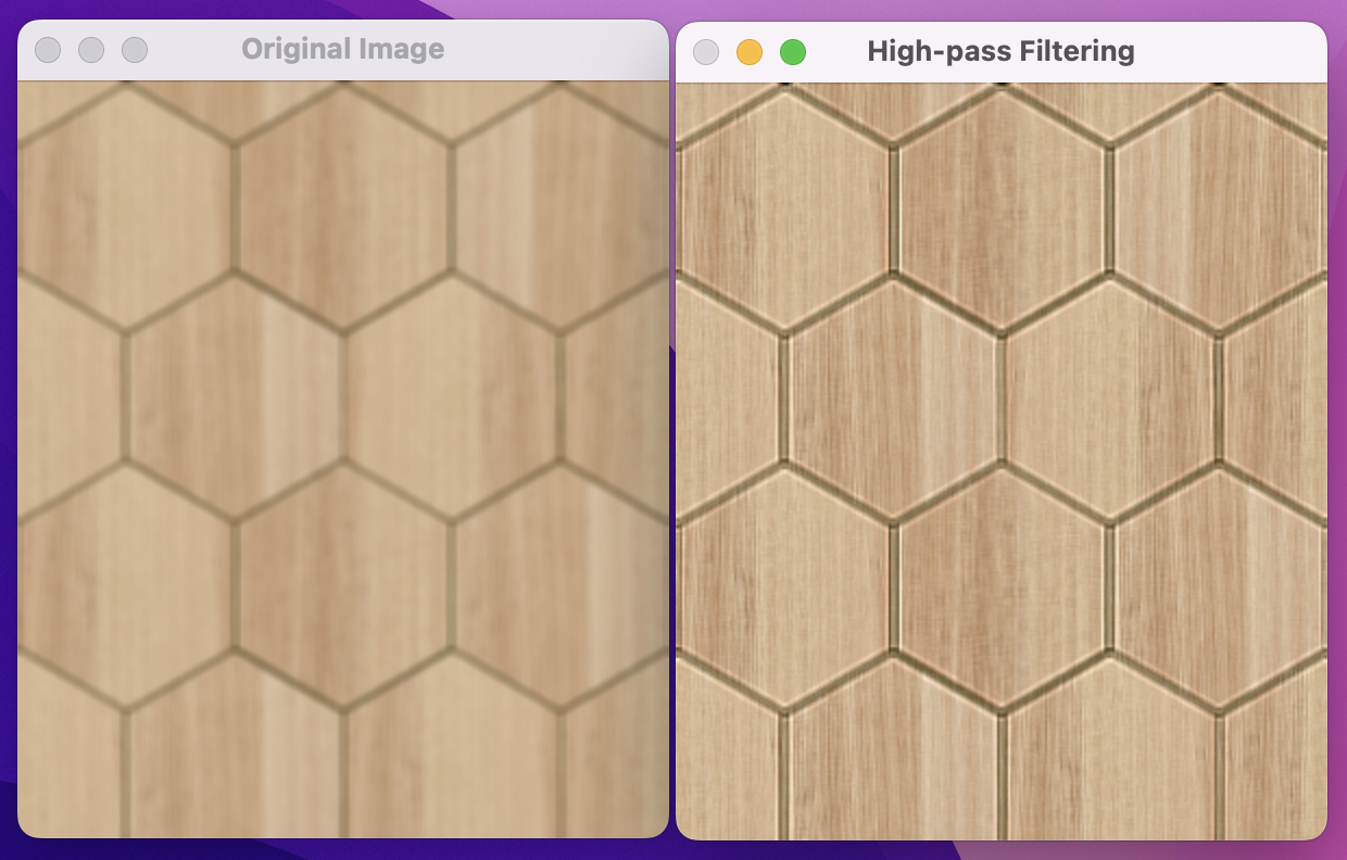
In the above code, we first read an image using cv2.imread(). Then, we define a kernel for high-pass filtering. This kernel is a 3x3 matrix that emphasizes the center pixel and suppresses the surrounding pixels. We then apply the high-pass filter using cv2.filter2D(), and finally display the result using cv2.imshow().

b. Unsharp Masking

Another common technique for image sharpening is unsharp masking. This technique works by blurring the image and then subtracting the blurred image from the original image. This can be achieved using the cv2.addWeighted() function. The result is an image that is sharper than the original.

import cv2
import numpy as np

# Read an image
img = cv2.imread("zidane.jpg")

# Apply gaussian blur
blurred = cv2.GaussianBlur(img, (7, 7), 0)

# Calculate the unsharp image
sharpened_img = cv2.addWeighted(img, 2.0, blurred, -1.0, 0)

# Display the results
cv2.imshow("Original Image", img)
cv2.imshow("Unsharp Masking", sharpened_img)
cv2.waitKey(0)
cv2.destroyAllWindows()

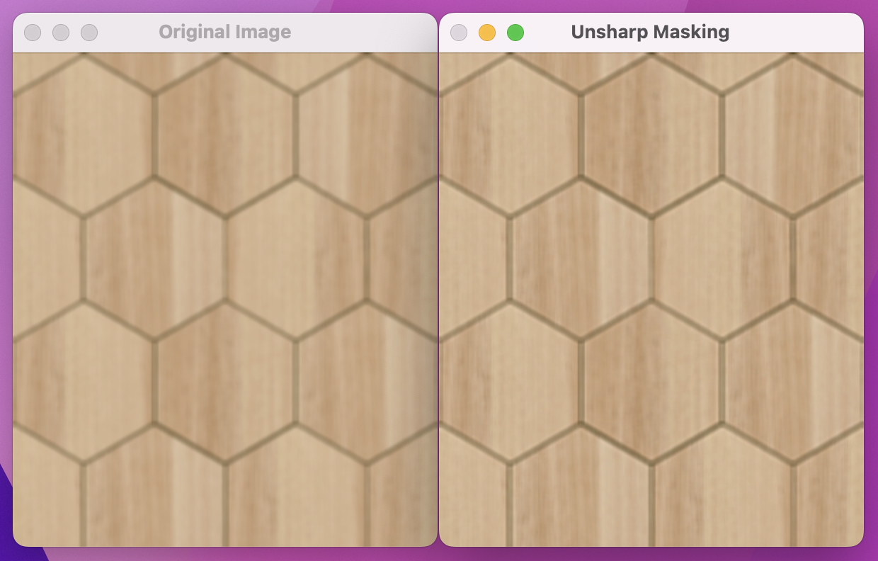
First, the code reads an input image using the cv2.imread() function and stores it in the variable img.

Next, a Gaussian blur is applied to the input image using the cv2.GaussianBlur() function. The GaussianBlur() function takes three arguments: the input image, the kernel size, and the standard deviation in the x and y directions. In this case, a kernel size of (7, 7) and a standard deviation of 0 are used to apply the blur. The blurred image is stored in the variable blurred.

Then, the unsharp image is calculated using the cv2.addWeighted() function. This function takes five arguments: the input image, the weight to be applied to the input image, the blurred image, the weight to be applied to the blurred image, and a scalar offset value. In this case, the input image is multiplied by a weight of 2.0, and the blurred image is multiplied by a weight of -1.0. These values are added together, and the resulting image is stored in the variable sharpened_img.

c. Laplacian Operator

Laplacian filter is another technique used for edge detection and image sharpening. The filter highlights the edges in an image by calculating the second derivative of the image. In OpenCV, we can achieve this using the cv2.Laplacian() function.

import cv2

# Read an image
img = cv2.imread("wood_blur.png")

# Apply Laplacian filter
laplacian = cv2.Laplacian(img, cv2.CV_64F)

# Add the Laplacian filter output to the original image
sharpened_img = cv2.add(img, laplacian, dtype=cv2.CV_8UC3)

# Display the results
cv2.imshow("Original Image", img)
cv2.imshow("Sharpened Image", sharpened_img)
cv2.waitKey(0)
cv2.destroyAllWindows()

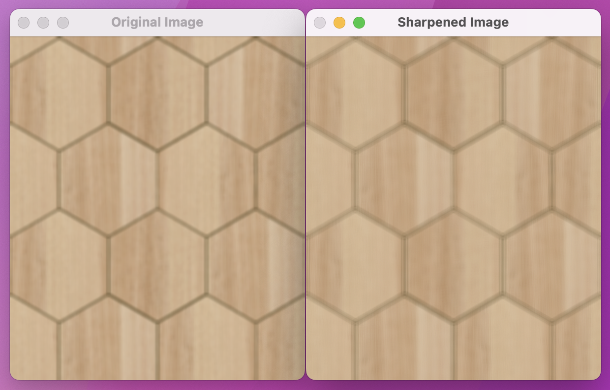
The above code applies the Laplacian filter to an input image using the cv2.Laplacian() function from the OpenCV library. The Laplacian filter is a type of edge detection filter that enhances the edges in an image. It works by calculating the second-order derivative of the image, which highlights the areas of the image where the intensity changes rapidly. The output of the Laplacian filter is then added to the original image using the cv2.add() function. The result is a sharpened image with enhanced edges.

Comparison: All Filters at a Glance

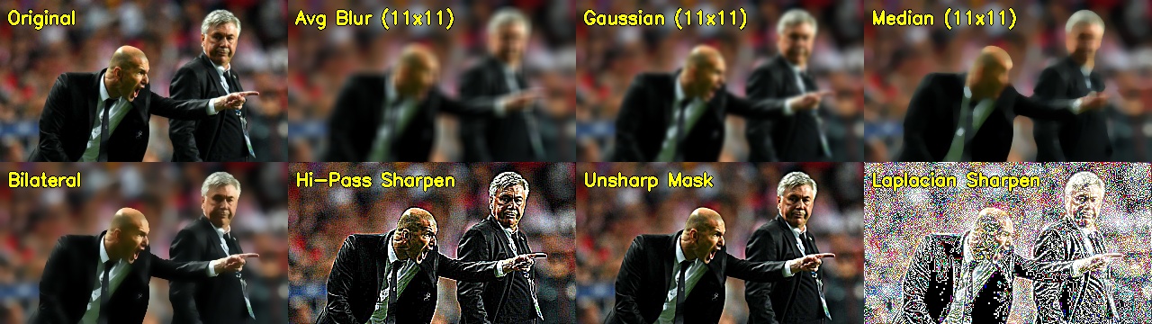
Run this to see all four blur types and two sharpening methods side-by-side on the portrait:

import cv2
import numpy as np
import urllib.request

urllib.request.urlretrieve("https://ultralytics.com/images/zidane.jpg", "zidane.jpg")
img = cv2.imread("zidane.jpg")
img = cv2.resize(img, (320, 240))

# Blur variants
avg     = cv2.blur(img, (9, 9))
gauss   = cv2.GaussianBlur(img, (9, 9), 0)
median  = cv2.medianBlur(img, 9)
bilat   = cv2.bilateralFilter(img, 9, 75, 75)

# Sharpen variants
kernel_hp = np.array([[-1,-1,-1],[-1, 9,-1],[-1,-1,-1]])
sharp_hp  = cv2.filter2D(img, -1, kernel_hp)
blurred   = cv2.GaussianBlur(img, (7, 7), 0)
sharp_um  = cv2.addWeighted(img, 2.0, blurred, -1.0, 0)

def label(im, text):
    out = im.copy()
    cv2.putText(out, text, (6, 22), cv2.FONT_HERSHEY_SIMPLEX, 0.55, (0,255,255), 1)
    return out

row1 = cv2.hconcat([label(img,     "Original"),
                    label(avg,     "Avg Blur"),
                    label(gauss,   "Gaussian"),
                    label(median,  "Median")])
row2 = cv2.hconcat([label(bilat,   "Bilateral"),
                    label(sharp_hp,"Hi-Pass Sharp"),
                    label(sharp_um,"Unsharp Mask"),
                    label(img,     "")])

grid = cv2.vconcat([row1, row2])
cv2.imshow("Filter Comparison (press any key to close)", grid)
cv2.waitKey(0)
cv2.destroyAllWindows()

# Expected:
# - Avg/Gaussian/Median: face smoothed, detail reduced
# - Bilateral: face smoothed but edges (jawline, eyes) stay sharp
# - Hi-pass / Unsharp: skin texture, hair strands more pronounced

Conclusion

Image filtering is a crucial preprocessing step in every CV pipeline. The bilateral filter is the gold standard when you need smooth regions but sharp boundaries — common in portrait retouching and semantic segmentation preprocessing. Edge detection, covered next, builds directly on these filtering concepts.